Anomaly Detection with New York City taxi data

In this entry, I will be conducting anomaly detection to identify points of anomaly in the taxi passengers data in New York City from July 2014 to January 2015 at half-hourly intervals.

(4 min read)

Introduction to Anomaly Detection

• Anomaly detection is an unsupervised machine learning technique that identifies outliers - a data point that differs from other majority data points - and their patterns in the data set. Such outliers could be a super hot day (as in 50 degree celcius) in the middle of winter with the average temperature of -10 degree Celcius. This technique can be used to detect outliers to remove in data preprocessing or even to identify potential frauds or failures in health system monitoring.

Dataset

• First off, we will load the dataset and the essential libraries as usual and read the first five rows to see what is going on. The output below shows that we have timestamp data and the number of passengers as indicated by the value column.

Show code

library(tidyverse) #for data manipulation
library(lubridate) #for date/time data management
library(zoo) # moving averages  
library(anomalize) #for anomaly detection

data <- read_csv("nyc_taxi.csv")
head(data)

# A tibble: 6 x 2
  timestamp           value
  <dttm>              <dbl>
1 2014-07-01 00:00:00 10844
2 2014-07-01 00:30:00  8127
3 2014-07-01 01:00:00  6210
4 2014-07-01 01:30:00  4656
5 2014-07-01 02:00:00  3820
6 2014-07-01 02:30:00  2873

• Let us visualize the data with ggplot2 to see what the data set is like before we proceed further.

Show code

ggplot(data, aes(x = timestamp, y = value)) + 
  geom_point(shape = 1, alpha = 0.5) +
  labs(x = "Time", y = "Count") +
  labs(alpha = "", colour="Legend")

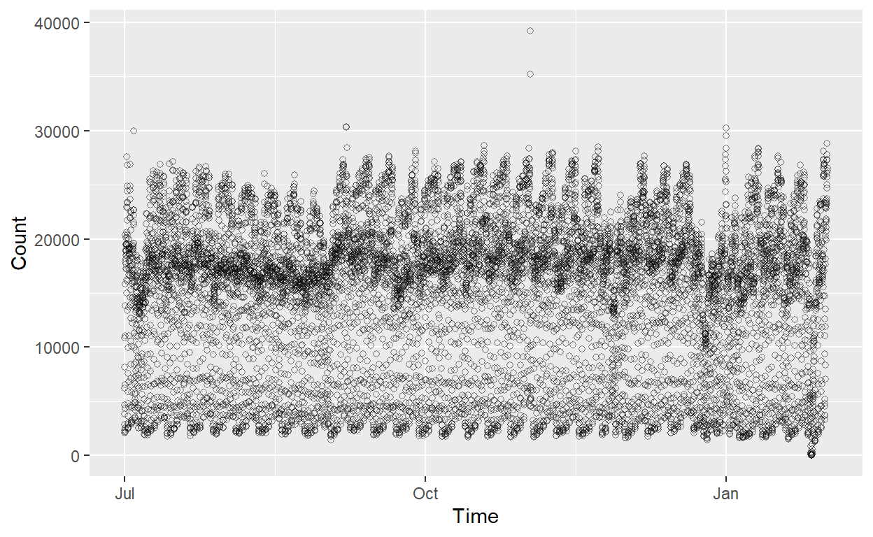
• Time series data is usually represented in patterns across time, but fluctuations could occur by the influence of events that affect the variable of interest such as holidays or natural phenomenon.

Investigating the Moving Average

• In simple word, a moving average is an indicator that shows the average value of the variable of interest over a period (i.e. 10 days, 50 days, 200 days, etc) and is usually plotted across a large time interval as in months or years.

• We will create two moving averages, one with 48 value in each group, and another one with 336 value in each group.

Show code

data <- data %>% 
  dplyr::mutate (MA48 = zoo::rollmean(value, k = 48, fill = NA),
                MA336 = zoo::rollmean(value, k = 336, fill = NA)) %>%
  dplyr::ungroup()

#Plot the moving average line chart

data %>%
  gather(metric, value, MA48:MA336) %>%
  ggplot(aes(timestamp, value, color = metric)) +
  geom_line() +
  ggtitle("Rolling average of NYC taxi passenger count")+
  theme(plot.title = element_text(hjust = 0.5))

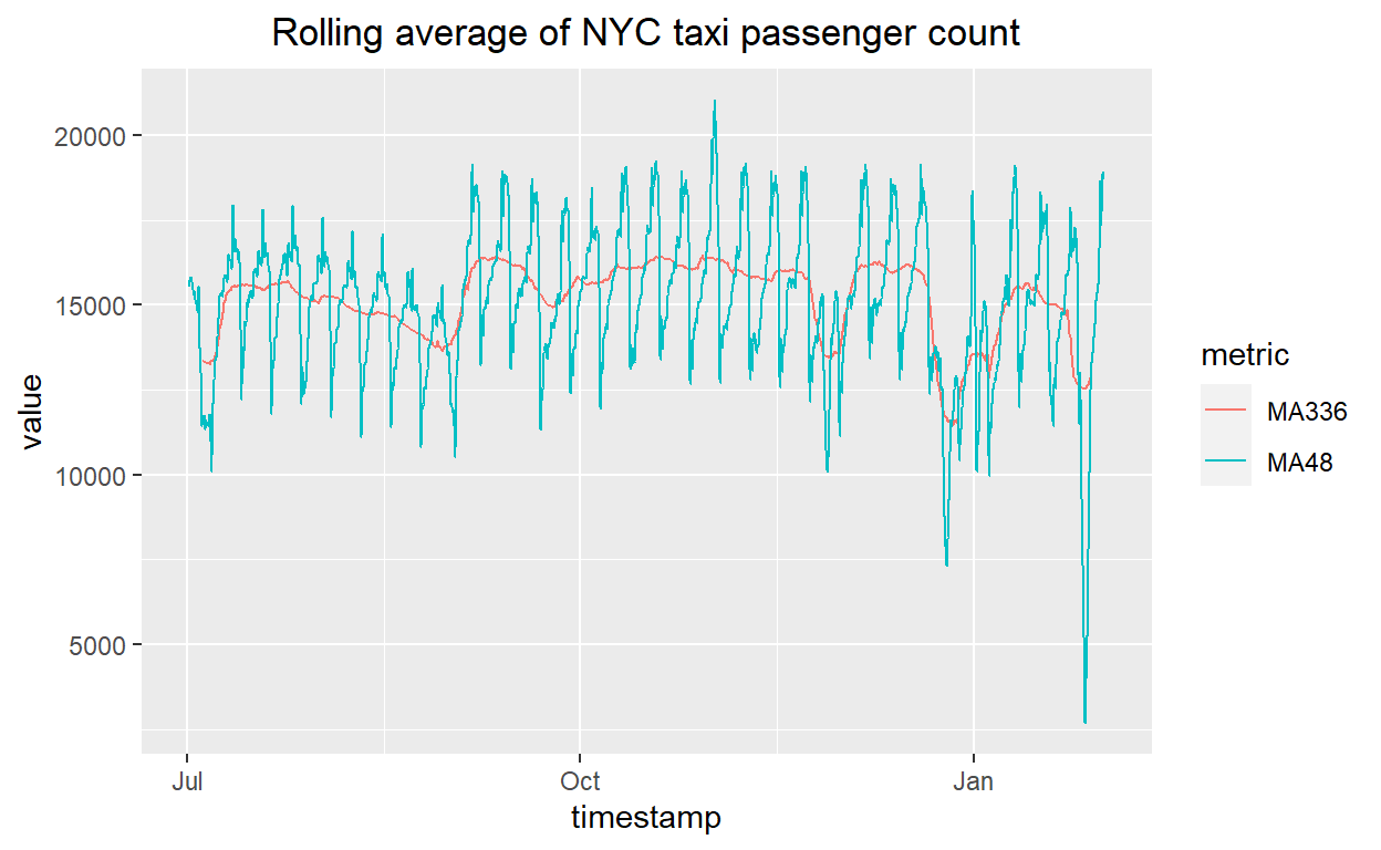
• We can see that the anomaly is more apparent when we divide the data into groups with 48 data points.

Time Series Decomposition with Anomalies

• Before we dive into anomaly detection, we should conduct time series decomposition where time series data is decomposed into Seasonal, Trend and remainder components with time_decompose().
  
• Once the components are decomposed, anomalize() can detect and flag anomalies in the decomposed data of the reminder component which then could be visualized with plot_anomaly_decomposition()

Show code

data %>% 
  time_decompose(value, method = "stl", frequency = "auto", trend = "auto") %>%
  anomalize(remainder, method = "gesd", alpha = 0.05, max_anoms = 0.2) %>%
  plot_anomaly_decomposition()

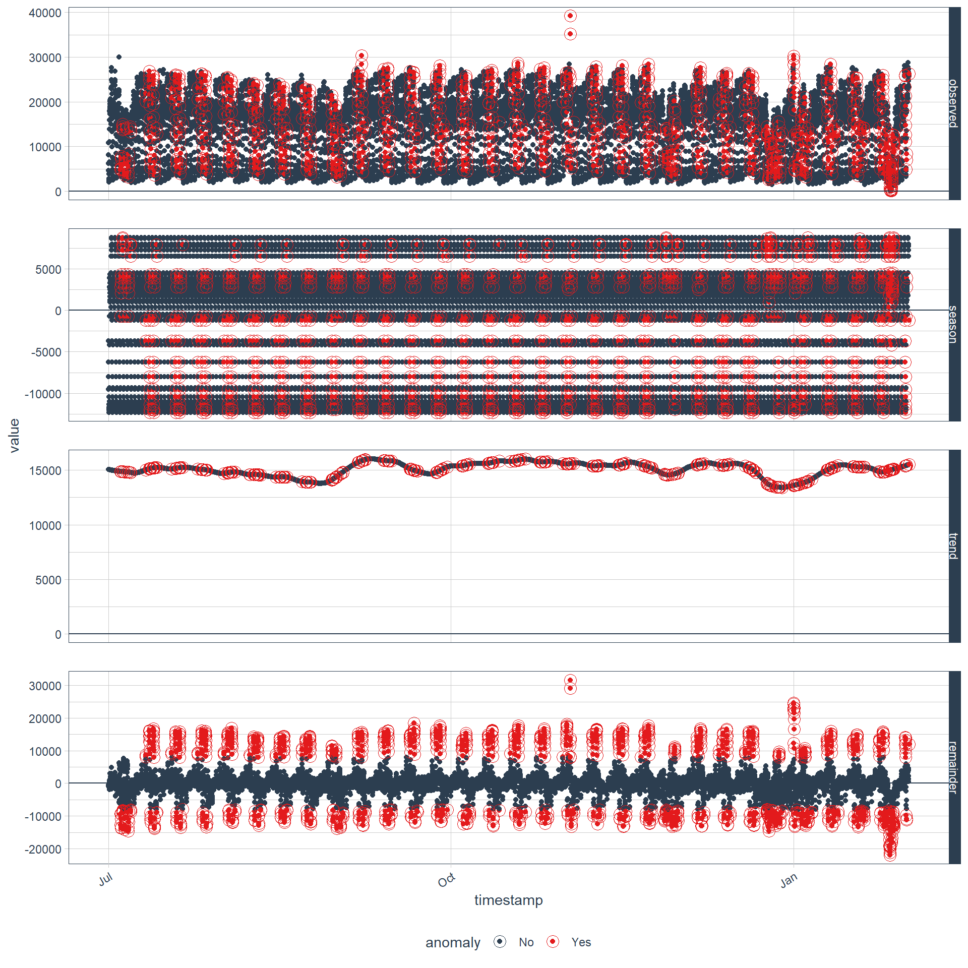
• For each element of the graph, observed represents the actual value, season represents the seasonal or cyclic trend, trend is a long term trend throughout the whole time period, and remainder is the observed data minus by results from season and trend.

Anomaly Detection

• Anomaly Detection and Plotting the detected anomalies are similar to the time series decomposition above, but we do not have to adjust parameters such as frequency, trend, or method like we did above. Basically, it is easier than time series decomposition as we can use it out of the box.

Show code

data %>% 
  time_decompose(value) %>%
  anomalize(remainder) %>%
  time_recompose() %>%
  plot_anomalies(time_recomposed = TRUE, ncol = 3, alpha_dots = 0.5)

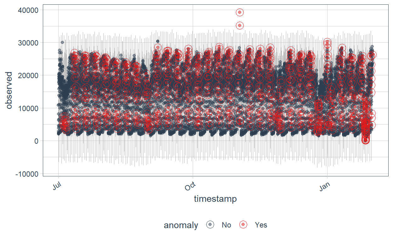
• Notice that the model has picked several anomalies around January, which contains the New Year festival and the occurrence of a blizzard storm at the New York City. Points of anomaly usually occurs with events of some sort, so we might be able to identify sources of anomaly with further information search using the date of anomaly as the lead.

• We can also extract the actual anomalous data point via the following codes:

Show code

data_anomalous <- data %>% 
  time_decompose(value) %>%
  anomalize(remainder) %>%
  time_recompose() %>%
  filter(anomaly == 'Yes') 

head(data_anomalous)

# A time tibble: 6 x 10
# Index: timestamp
  timestamp           observed season  trend remainder remainder_l1
  <dttm>                 <dbl>  <dbl>  <dbl>     <dbl>        <dbl>
1 2014-07-04 07:30:00     4926  2817. 14875.   -12767.       -9534.
2 2014-07-04 08:00:00     5165  3903. 14875.   -13612.       -9534.
3 2014-07-04 08:30:00     5776  4346. 14874.   -13445.       -9534.
4 2014-07-04 09:00:00     7338  3304. 14874.   -10840.       -9534.
5 2014-07-05 07:00:00     3658  -735. 14848.   -10454.       -9534.
6 2014-07-05 07:30:00     4345  2817. 14847.   -13319.       -9534.
# ... with 4 more variables: remainder_l2 <dbl>, anomaly <chr>,
#   recomposed_l1 <dbl>, recomposed_l2 <dbl>

• I know that the amount of detected anomaly is a lot. We can adjust parameter of the detector to make the algorithm less sensitive and detect stronger outliers by decreasing alpha and max_anoms to control for sensitivity and the maximum percentage of data that can be an anomaly respectively. max_anoms = 0.20 means the algorithm will flag anomalies up to 20% of the whole data set.

• The example above used default parameter, which is alpha = 0.05 and max_anoms = 0.20. Let us try tuning down the sensitivity a little bit, say, alpha = 0.025 and max_anoms = 0.05 to identify only extreme outliers.

Show code

data %>% 
  time_decompose(value) %>%
  anomalize(remainder, alpha = 0.025, max_anoms = 0.05) %>%
  time_recompose() %>%
  plot_anomalies(time_recomposed = TRUE, ncol = 3, alpha_dots = 0.5)

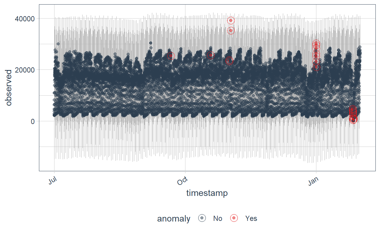
• Even with parameter tuning, the algorithm still detects anomalies at the end of January. Something must be going on there. Let us extract the actual anomalous data point of the tuned algorithm.

Show code

data_anomalous_tuned <- data %>% 
  time_decompose(value) %>%
  anomalize(remainder, alpha = 0.025, max_anoms = 0.05) %>%
  time_recompose() %>%
  filter(anomaly == 'Yes') 

head(data_anomalous_tuned)

# A time tibble: 6 x 10
# Index: timestamp
  timestamp           observed  season  trend remainder remainder_l1
  <dttm>                 <dbl>   <dbl>  <dbl>     <dbl>        <dbl>
1 2014-09-21 01:00:00    25371  -8034. 14994.    18411.      -17691.
2 2014-10-19 01:00:00    25610  -8034. 15905.    17739.      -17691.
3 2014-11-01 01:30:00    23736  -9536. 15566.    17707.      -17691.
4 2014-11-01 02:00:00    23245 -10442. 15565.    18121.      -17691.
5 2014-11-02 01:00:00    39197  -8034. 15597.    31634.      -17691.
6 2014-11-02 01:30:00    35212  -9536. 15598.    29151.      -17691.
# ... with 4 more variables: remainder_l2 <dbl>, anomaly <chr>,
#   recomposed_l1 <dbl>, recomposed_l2 <dbl>

Application of Anomaly Detection

• Anomaly detection has wide applications across industries. Data scientists can identify anomalies in the amount of deposits that go outside the usual pattern, thus flagging it for potential fraud or system error for a deeper investigation. The technique can also be used to identify anomalous data in student pattern from their e-learning platform, which could lead us to topics that can be further explored such as a fluctuation in the duration of content access. A certain content could be exceedingly difficult that students have to spend more time than usual studying it.

• Aside from using R, anomaly can also be done in Python as well. If you are interested, you can check out my Jupyter notebook here for anomaly detection with Pycaret, a low-code machine learning library in Python that covers end-to-end machine learning pipeline from preprocessing to model deploying. Thank you very much for reading!