Applying Machine Learning to Audio Data: Visualization, Classification, and Recommendation

For this entry, I am trying my hands on audio data to extract its features for exploratory data analysis (EDA), using machine learning algorithms to perform music classification, and finally build up on that result to develop a recommendation system for music of similar characteristics.

(13 min read)

Machine Learning with Audio data

• When we think of data, people may think of numbers and texts in tables. Some may even think of using images as data, but just so you know, we can also convert and extract features from audio data (i.e., music) to understand and make use of it as well! Here, we will visualize music sound wave from .wav files to understand about what differentiates one tone from another (we can actually see soundwaves!).

• I primarily relied on Olteanu et al. (2019)’s work, Music genre classification article, and Analytics Vidhya guide to the same topic to guide this reproduction and experimentation with the data.

• To introduce the data set a bit. I will be using the GTZAN dataset, which is a public data set for evaluation in machine listening research for music genre recognition (MGR). The files were collected in 2000-2001 from a variety of sources including personal CDs, radio, microphone recordings to represent a variety of recording conditions.

• We will start from importing audio data into our Python environment for data visualization; then, we will explore its feature such as sound wave, spectogram, mel-spectogram, harmonics and perceptrual, tempo, spectral centroid, and chroma frequencies. We will then conduct an exploratory data analysis with correlation heatmap with the extracted features, generating a box plot for genres distribution, and perform a principal component analysis to divide genres into groups.

• Lastly, we will perform machine learning classification to train the algorithm to recognize and predict new audio files into genres (e.g., rock, pop, jazz), as well as develop a music recommendation system using the cosine similarity statistics. This function is a part of music delivery platforms such as Spotify, Youtube music, or Apple Music.

• We will begin by importing necessary libraries for graphing (seaborn and matplotlib), data manipulation (pandas), machine learning (sklearn), and audio work (librosa).

Show code

# Usual Libraries
import pandas as pd
import numpy as np
import seaborn as sns
import matplotlib.pyplot as plt
import sklearn

import librosa
import librosa.display

Explore Audio Data

• We will use librosa, which is the main library for audio work in Python. Let us first Explore our Audio Data to see how it looks (we’ll work with pop.00002.wav file). We will check for sound - the sequence of vibrations in varying pressure strengths (y) and sample rate (sr) the number of samples of audio carried per second, measured in Hz or kHz.

Show code

# Importing 1 file
y, sr = librosa.load('D:/Program/Private_project/DistillSite/_posts/2021-12-11-applying-machine-learning-to-audio-data/genres_original/pop/pop.00002.wav')

print('y:', y, '\n')

y: [-0.09274292 -0.11630249 -0.11886597 ...  0.14419556  0.16311646
  0.09634399] 

Show code

print('y shape:', np.shape(y), '\n')

y shape: (661504,) 

Show code

print('Sample Rate (KHz):', sr, '\n')

# Verify length of the audio

Sample Rate (KHz): 22050 

Show code

print('Check Length of the audio in second:', 661794/22050)

Check Length of the audio in second: 30.013333333333332

• We will then clean the data by trimming all leading and trailing silence from the audio signal.

Show code

# Trim leading and trailing silence from an audio signal (silence before and after the actual audio)
audio_file, _ = librosa.effects.trim(y)

# the result is an numpy ndarray
print('Audio File:', audio_file, '\n')

Audio File: [-0.09274292 -0.11630249 -0.11886597 ...  0.14419556  0.16311646
  0.09634399] 

Show code

print('Audio File shape:', np.shape(audio_file))

Audio File shape: (661504,)

2D Representation: Sound Waves

• We can view a 2D representation of a sound with sound waves

Show code

plt.figure(figsize = (16, 6))

<Figure size 1600x600 with 0 Axes>

Show code

librosa.display.waveplot(y = audio_file, sr = sr, color = "#A300F9");
plt.title("Sound Waves in Pop 02", fontsize = 23);
plt.show()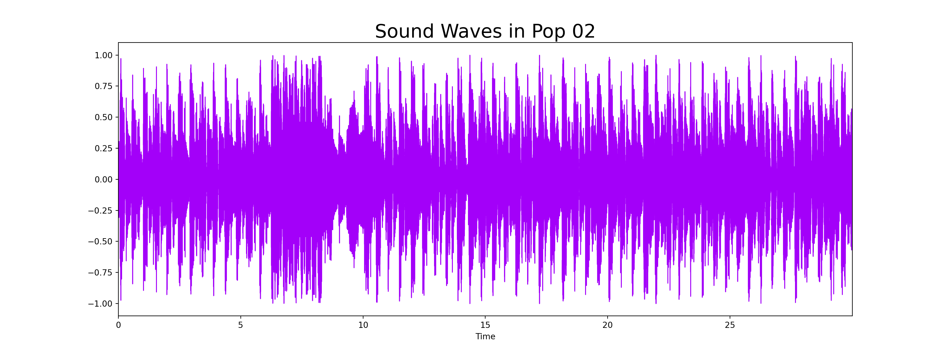

Fourier Transform

• We will then perform a fourier transform to convert the y-axis (frequency) to log scale, and the “color” axis (amplitude) to Decibels.

Show code

# Default FFT window size
n_fft = 2048 # FFT window size
hop_length = 512 # number audio of frames between STFT columns (looks like a good default)

# Short-time Fourier transform (STFT)
D = np.abs(librosa.stft(audio_file, n_fft = n_fft, hop_length = hop_length))

print('Shape of D object:', np.shape(D))

Shape of D object: (1025, 1293)

Show code

plt.figure(figsize = (16, 6))

<Figure size 1600x600 with 0 Axes>

Show code

plt.plot(D);
plt.show()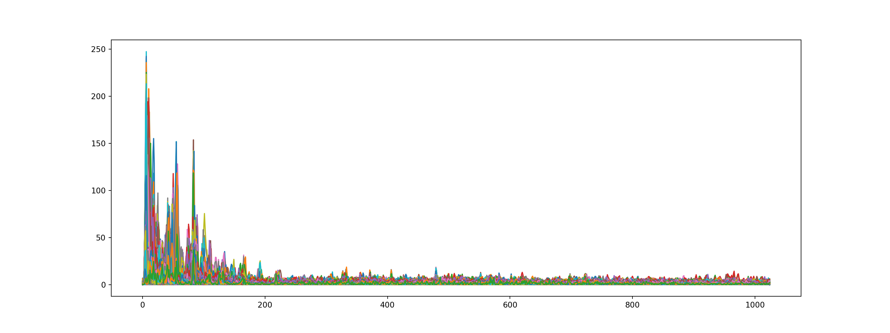

The Spectrogram

• Another characteristics that can represent a sound is its spectogram - a visual representation of signal frequencies across time (aka sonographs, voiceprints, or voicegrams).

Show code

# Convert an amplitude spectrogram to Decibels-scaled spectrogram.
DB = librosa.amplitude_to_db(D, ref = np.max)

# Creating the Spectogram
plt.figure(figsize = (16, 6))

<Figure size 1600x600 with 0 Axes>

Show code

librosa.display.specshow(DB, sr = sr, hop_length = hop_length, x_axis = 'time', y_axis = 'log', cmap = 'cool')

<matplotlib.collections.QuadMesh object at 0x000000006FAB1310>

Show code

plt.colorbar();
plt.show()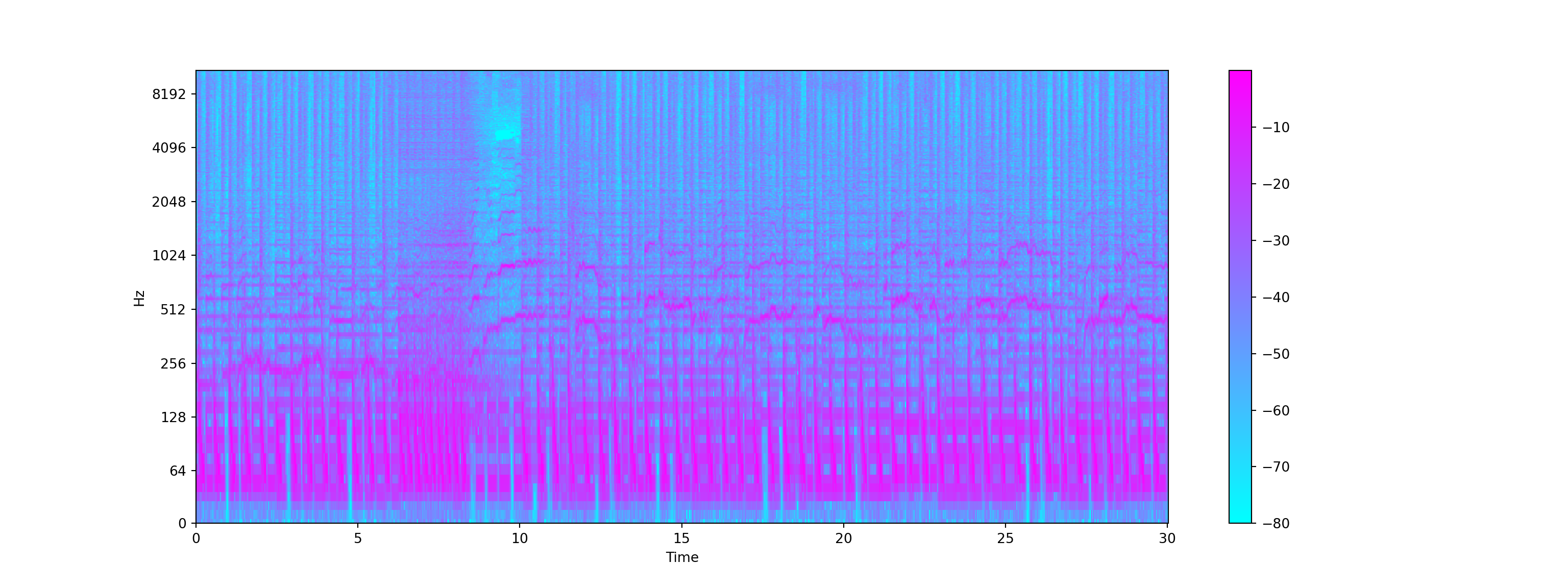

Mel Spectrogram

• The Mel Spectogram is a non-linear version of spectogram with a Mel scale on the y-axis. Mel scale converts the normal specrogram to frequencies that are perceptible by human ears, so basically, the difference between spectogram and mel spectogram is in its mathematical structure and its ability to be perceived by human. Each music genre has different spectogram (and mel spectogram) structure.

Show code

y, sr = librosa.load('D:/Program/Private_project/DistillSite/_posts/2021-12-11-applying-machine-learning-to-audio-data/genres_original/metal/metal.00036.wav')
y, _ = librosa.effects.trim(y)


S = librosa.feature.melspectrogram(y, sr=sr)
S_DB = librosa.amplitude_to_db(S, ref=np.max)
plt.figure(figsize = (16, 6))

<Figure size 1600x600 with 0 Axes>

Show code

librosa.display.specshow(S_DB, sr=sr, hop_length=hop_length, x_axis = 'time', y_axis = 'log',
                        cmap = 'cool');
plt.colorbar();
plt.title("Metal Mel Spectrogram", fontsize = 23);
plt.show()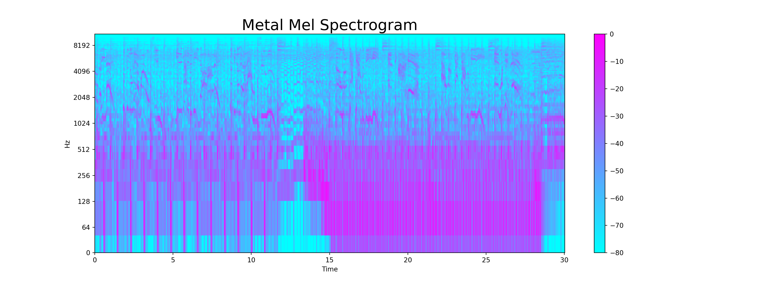

Show code

y, sr = librosa.load('D:/Program/Private_project/DistillSite/_posts/2021-12-11-applying-machine-learning-to-audio-data/genres_original/classical/classical.00036.wav')
y, _ = librosa.effects.trim(y)


S = librosa.feature.melspectrogram(y, sr=sr)
S_DB = librosa.amplitude_to_db(S, ref=np.max)
plt.figure(figsize = (16, 6))

<Figure size 1600x600 with 0 Axes>

Show code

librosa.display.specshow(S_DB, sr=sr, hop_length=hop_length, x_axis = 'time', y_axis = 'log',
                        cmap = 'cool');
plt.colorbar();
plt.title("Classical Mel Spectrogram", fontsize = 23);
plt.show()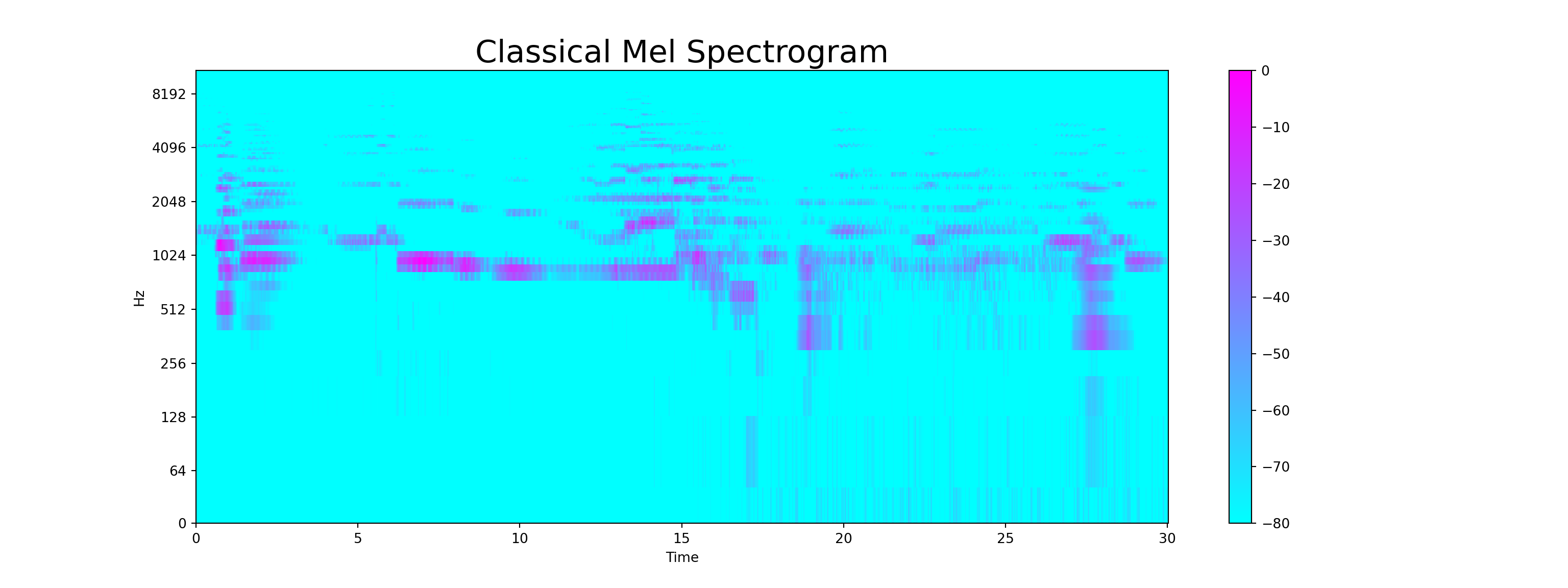

Audio Features

• Now that we have explored an audio file with several visualizations of Spectogram, fourier transform, and sound waves, let us try extracting audio features that we may use with data manipulation and machine learning.

Zero Crossing Rate

• the rate at which the sound signal changes from positive to negative and vice versa. This feature is usually used for speech recognition and music information retrieval. Music genre with high percussive sound like rock or metal usually have high Zero Crossing Rate than other genres.

Show code

# Total zero_crossings in our 1 song
zero_crossings = librosa.zero_crossings(audio_file, pad=False)
print(sum(zero_crossings))

78769

Harmonics and Perceptual

• Harmonics (the orange wave) are audio characteristics that human ears can’t distinguish (represents the sound color)

• Perceptual (the purple wave) are sound waves that represent rhythm and emotion of the music.

Show code

y_harm, y_perc = librosa.effects.hpss(audio_file)

plt.figure(figsize = (16, 6))

<Figure size 1600x600 with 0 Axes>

Show code

plt.plot(y_harm, color = '#A300F9');
plt.plot(y_perc, color = '#FFB100');
plt.show()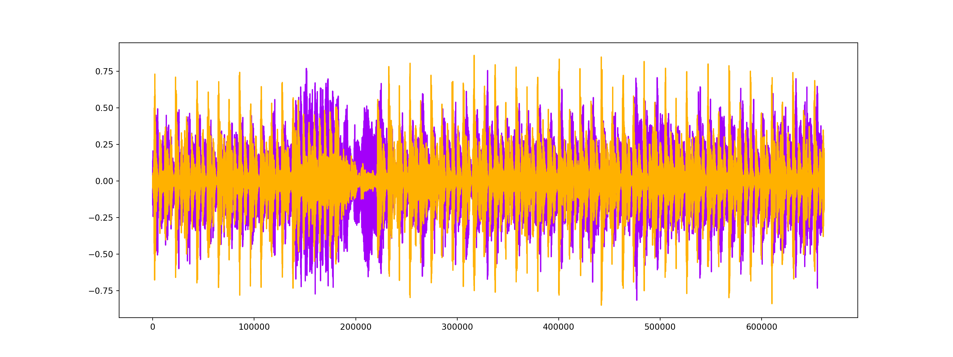

Tempo BMP (beats per minute)

• Tempo is the number of beat per one minute.

Show code

tempo, _ = librosa.beat.beat_track(y, sr = sr)
tempo

107.666015625

Spectral Centroid

• This variable represents brightness of a sound by calculating the center of sound spectrum (where the sound signal is at its peak). We can also plot it into a wave form.

Show code

# Calculate the Spectral Centroids
spectral_centroids = librosa.feature.spectral_centroid(audio_file, sr=sr)[0]

# Shape is a vector
print('Centroids:', spectral_centroids, '\n')

Centroids: [3042.39242043 3057.96296504 3043.45666379 ... 3476.4010229  3908.31319501
 3834.930348  ] 

Show code

print('Shape of Spectral Centroids:', spectral_centroids.shape, '\n')

# Computing the time variable for visualization

Shape of Spectral Centroids: (1293,) 

Show code

frames = range(len(spectral_centroids))

# Converts frame counts to time (seconds)
t = librosa.frames_to_time(frames)

print('frames:', frames, '\n')

frames: range(0, 1293) 

Show code

print('t:', t)

# Function that normalizes the Sound Data

t: [0.00000000e+00 2.32199546e-02 4.64399093e-02 ... 2.99537415e+01
 2.99769615e+01 3.00001814e+01]

Show code

def normalize(x, axis=0):
    return sklearn.preprocessing.minmax_scale(x, axis=axis)

Show code

#Plotting the Spectral Centroid along the waveform
plt.figure(figsize = (16, 6))

<Figure size 1600x600 with 0 Axes>

Show code

librosa.display.waveplot(audio_file, sr=sr, alpha=0.4, color = '#A300F9');
plt.plot(t, normalize(spectral_centroids), color='#FFB100');
plt.show()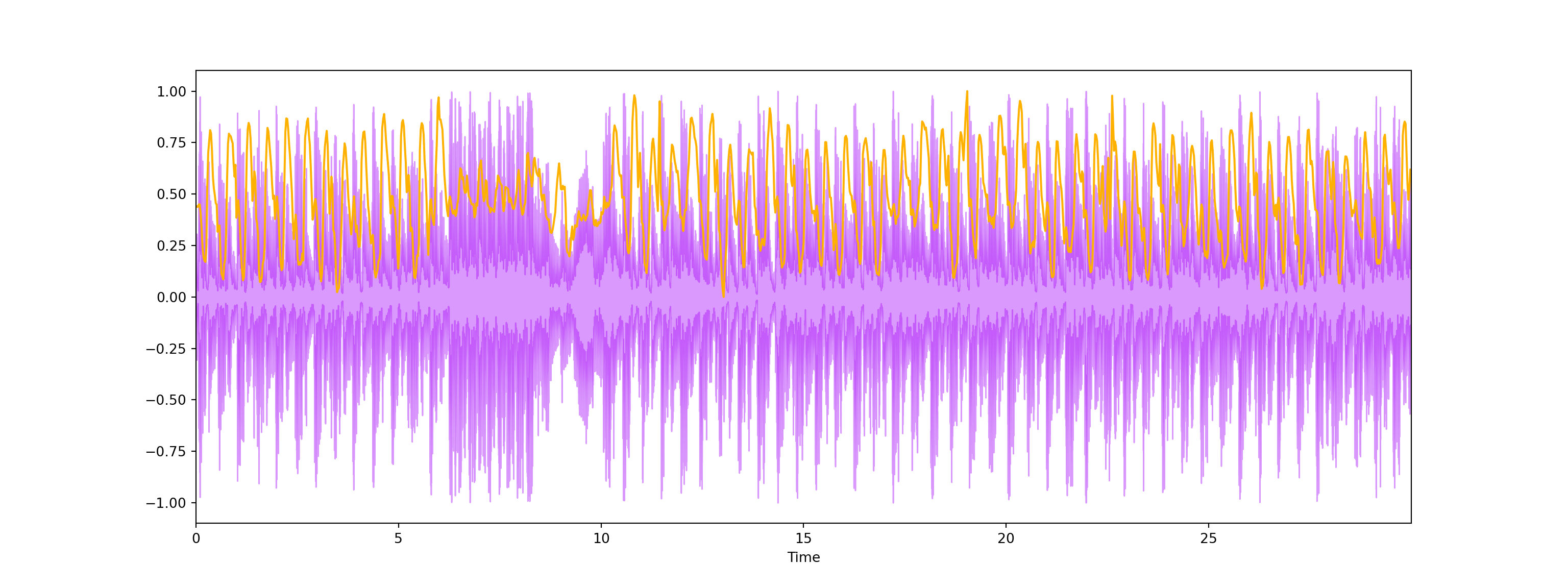

Spectral Rolloff

• Spectral Rolloff is a frequency below a specified percentage of the total spectral energy. It is like we have a cut-point, and we visualize the sound wave that is below that cut-point. Let’s just call it as another characteristic of a sound.

Show code

# Spectral RollOff Vector
spectral_rolloff = librosa.feature.spectral_rolloff(audio_file, sr=sr)[0]

# The plot
plt.figure(figsize = (16, 6))

<Figure size 1600x600 with 0 Axes>

Show code

librosa.display.waveplot(audio_file, sr=sr, alpha=0.4, color = '#A300F9');
plt.plot(t, normalize(spectral_rolloff), color='#FFB100');
plt.show()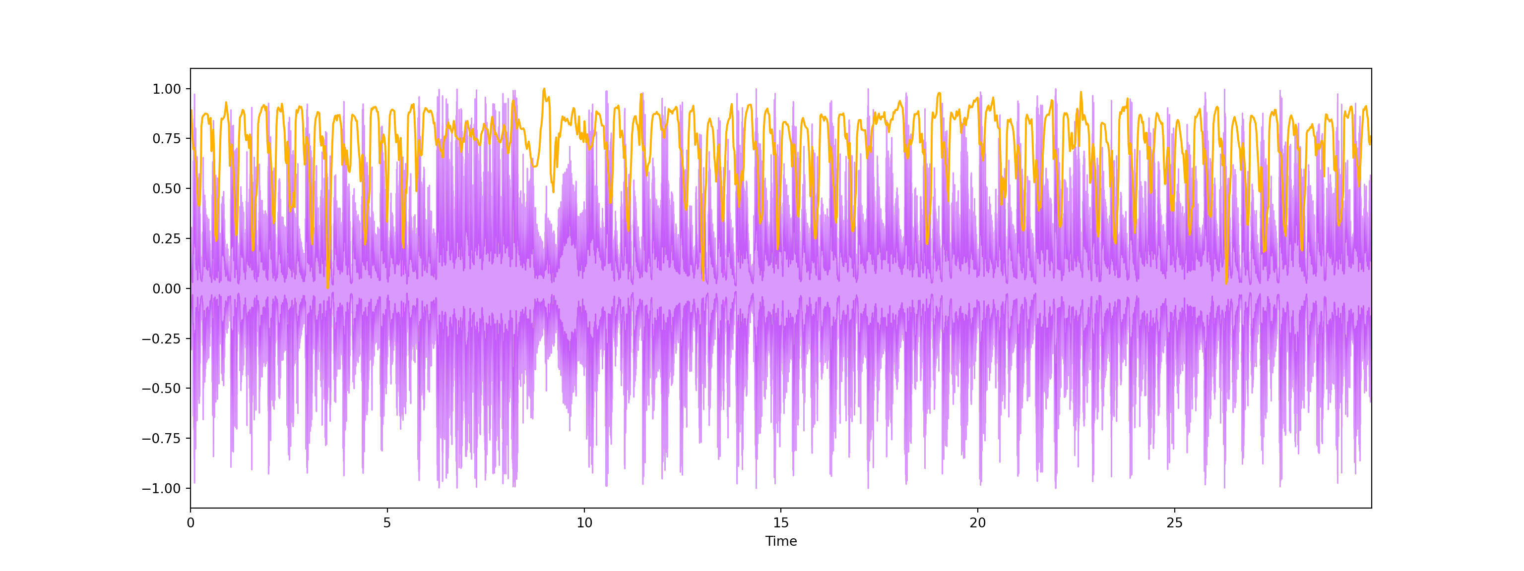

Mel-Frequency Cepstral Coefficients

• The Mel frequency Cepstral coefficients (MFCCs) of a signal are a small set of features that describes the overall shape of a spectral envelope. It imitates characteristics of human voice.

Show code

mfccs = librosa.feature.mfcc(audio_file, sr=sr)
print('mfccs shape:', mfccs.shape)

#Displaying  the MFCCs:

mfccs shape: (20, 1293)

Show code

plt.figure(figsize = (16, 6))

<Figure size 1600x600 with 0 Axes>

Show code

librosa.display.specshow(mfccs, sr=sr, x_axis='time', cmap = 'cool');
plt.show()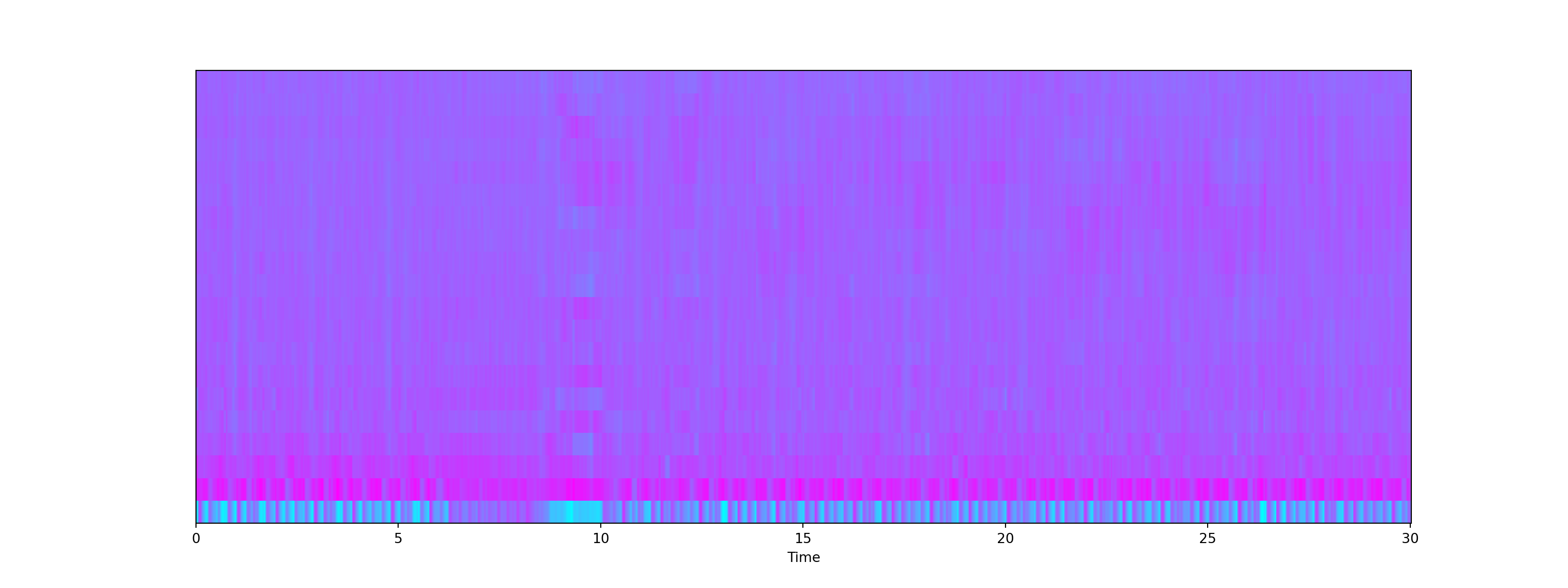

• We can scale the data a bit to make the feature (blue part) more apparent.

Show code

# Perform Feature Scaling
mfccs = sklearn.preprocessing.scale(mfccs, axis=1)

C:\Users\tarid\AppData\Roaming\Python\Python38\site-packages\sklearn\preprocessing\_data.py:174: UserWarning: Numerical issues were encountered when centering the data and might not be solved. Dataset may contain too large values. You may need to prescale your features.
  warnings.warn("Numerical issues were encountered "
C:\Users\tarid\AppData\Roaming\Python\Python38\site-packages\sklearn\preprocessing\_data.py:191: UserWarning: Numerical issues were encountered when scaling the data and might not be solved. The standard deviation of the data is probably very close to 0. 
  warnings.warn("Numerical issues were encountered "

Show code

print('Mean:', mfccs.mean(), '\n')

Mean: 3.097782e-09 

Show code

print('Var:', mfccs.var())

Var: 1.0

Show code

plt.figure(figsize = (16, 6))

<Figure size 1600x600 with 0 Axes>

Show code

librosa.display.specshow(mfccs, sr=sr, x_axis='time', cmap = 'cool');
plt.show()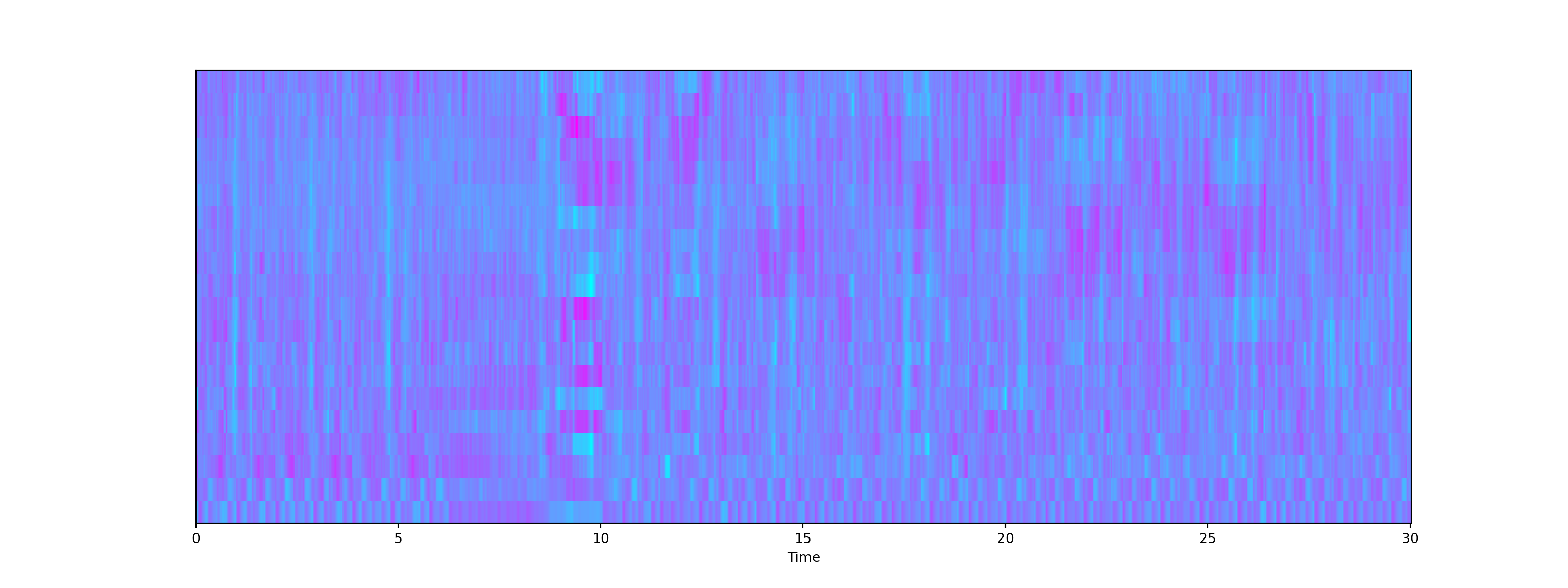

Chroma Frequencies

• Chroma feature represents the tone of music or sound by projecting its sound spectrum into a space that represents musical octave. This feature is usually used in chord recognition task.

Show code

# Increase or decrease hop_length to change how granular you want your data to be
hop_length = 5000

# Chromogram
chromagram = librosa.feature.chroma_stft(audio_file, sr=sr, hop_length=hop_length)
print('Chromogram shape:', chromagram.shape)

Chromogram shape: (12, 133)

Show code

plt.figure(figsize=(16, 6))

<Figure size 1600x600 with 0 Axes>

Show code

librosa.display.specshow(chromagram, x_axis='time', y_axis='chroma', hop_length=hop_length, cmap='coolwarm');
plt.show()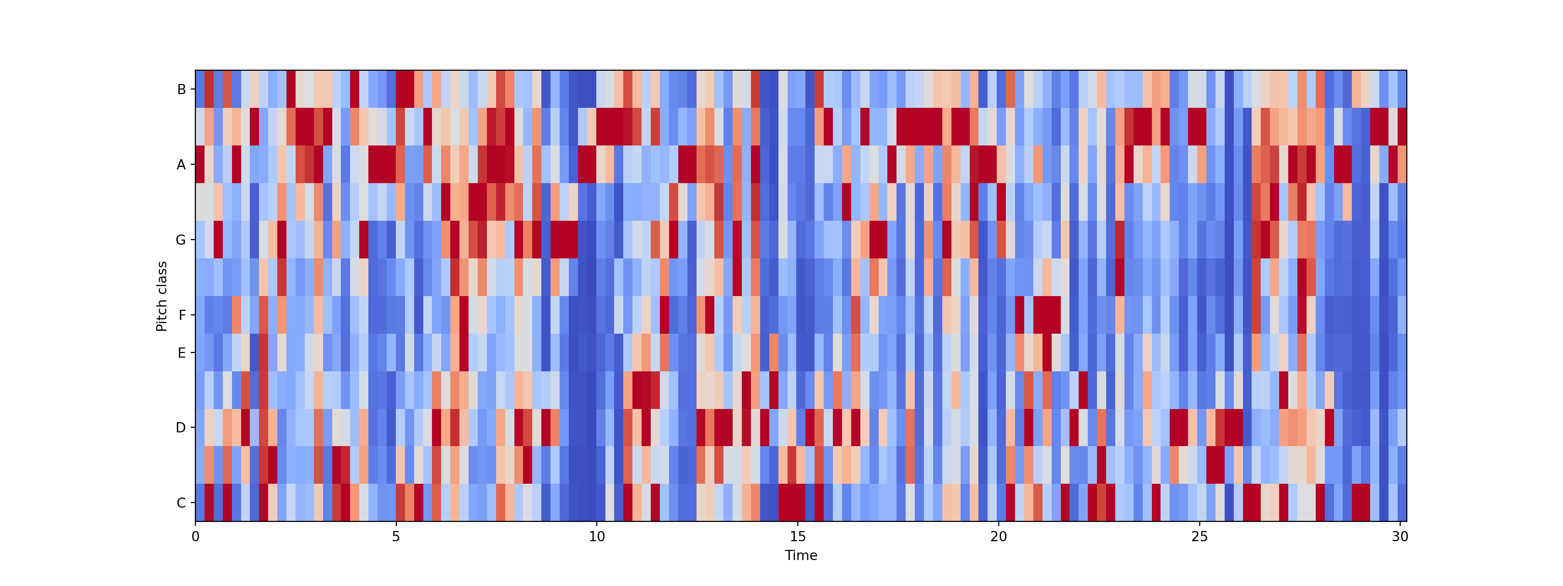

Exploratory Data Analysis

• We will perform an exploratory data analysis with the features_30_sec.csv data that contains the mean and variance of the features discussed above for all audio file in the data bank. We have 10 genres of music, each genre has 100 audio files. That makes the total of 1000 songs that we have. There are 60 features in total for each song.

Show code

data = pd.read_csv('features_30_sec.csv')
data.head()

          filename  length  chroma_stft_mean  ...  mfcc20_mean  mfcc20_var  label
0  blues.00000.wav  661794          0.350088  ...     1.221291   46.936035  blues
1  blues.00001.wav  661794          0.340914  ...     0.531217   45.786282  blues
2  blues.00002.wav  661794          0.363637  ...    -2.231258   30.573025  blues
3  blues.00003.wav  661794          0.404785  ...    -3.407448   31.949339  blues
4  blues.00004.wav  661794          0.308526  ...   -11.703234   55.195160  blues

[5 rows x 60 columns]

Correlation Heatmap for feature means

• Here, we are making a correlation heatmap among feature means to see which feature correlates with which. The redder a square is, the more negative the correlation between that pair of variable becomes.

Show code

# Computing the Correlation Matrix
spike_cols = [col for col in data.columns if 'mean' in col]
corr = data[spike_cols].corr()

# Generate a mask for the upper triangle
mask = np.triu(np.ones_like(corr, dtype=np.bool))

# Set up the matplotlib figure
f, ax = plt.subplots(figsize=(16, 11));

# Generate a custom diverging colormap
cmap = sns.diverging_palette(0, 25, as_cmap=True, s = 90, l = 45, n = 5)

# Draw the heatmap with the mask and correct aspect ratio
sns.heatmap(corr, mask=mask, cmap=cmap, vmax=.3, center=0,
            square=True, linewidths=.5, cbar_kws={"shrink": .5})

<AxesSubplot:>

Show code

plt.title('Correlation Heatmap (for the MEAN variables)', fontsize = 25)

Text(0.5, 1.0, 'Correlation Heatmap (for the MEAN variables)')

Show code

plt.xticks(fontsize = 10)

(array([ 0.5,  1.5,  2.5,  3.5,  4.5,  5.5,  6.5,  7.5,  8.5,  9.5, 10.5,
       11.5, 12.5, 13.5, 14.5, 15.5, 16.5, 17.5, 18.5, 19.5, 20.5, 21.5,
       22.5, 23.5, 24.5, 25.5, 26.5, 27.5]), [Text(0.5, 0, 'chroma_stft_mean'), Text(1.5, 0, 'rms_mean'), Text(2.5, 0, 'spectral_centroid_mean'), Text(3.5, 0, 'spectral_bandwidth_mean'), Text(4.5, 0, 'rolloff_mean'), Text(5.5, 0, 'zero_crossing_rate_mean'), Text(6.5, 0, 'harmony_mean'), Text(7.5, 0, 'perceptr_mean'), Text(8.5, 0, 'mfcc1_mean'), Text(9.5, 0, 'mfcc2_mean'), Text(10.5, 0, 'mfcc3_mean'), Text(11.5, 0, 'mfcc4_mean'), Text(12.5, 0, 'mfcc5_mean'), Text(13.5, 0, 'mfcc6_mean'), Text(14.5, 0, 'mfcc7_mean'), Text(15.5, 0, 'mfcc8_mean'), Text(16.5, 0, 'mfcc9_mean'), Text(17.5, 0, 'mfcc10_mean'), Text(18.5, 0, 'mfcc11_mean'), Text(19.5, 0, 'mfcc12_mean'), Text(20.5, 0, 'mfcc13_mean'), Text(21.5, 0, 'mfcc14_mean'), Text(22.5, 0, 'mfcc15_mean'), Text(23.5, 0, 'mfcc16_mean'), Text(24.5, 0, 'mfcc17_mean'), Text(25.5, 0, 'mfcc18_mean'), Text(26.5, 0, 'mfcc19_mean'), Text(27.5, 0, 'mfcc20_mean')])

Show code

plt.yticks(fontsize = 10);
plt.show()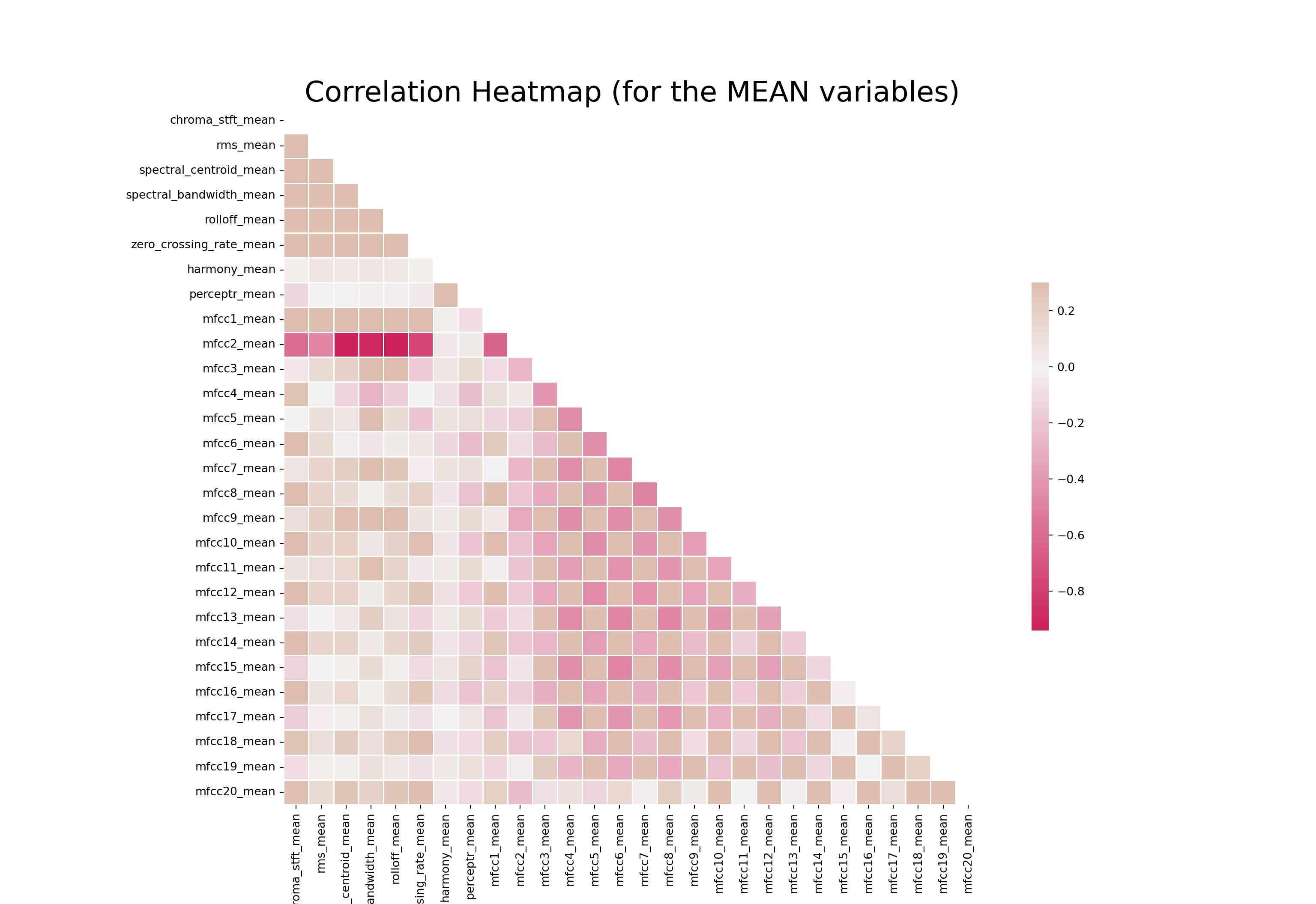

Box Plot for Genres Distributions

• We will also make a boxplot for tempo of all music genres.

Show code

x = data[["label", "tempo"]]

f, ax = plt.subplots(figsize=(16, 9));
sns.boxplot(x = "label", y = "tempo", data = x, palette = 'husl');

plt.title('BPM Boxplot for Genres', fontsize = 25)

Text(0.5, 1.0, 'BPM Boxplot for Genres')

Show code

plt.xticks(fontsize = 14)

(array([0, 1, 2, 3, 4, 5, 6, 7, 8, 9]), [Text(0, 0, 'blues'), Text(1, 0, 'classical'), Text(2, 0, 'country'), Text(3, 0, 'disco'), Text(4, 0, 'hiphop'), Text(5, 0, 'jazz'), Text(6, 0, 'metal'), Text(7, 0, 'pop'), Text(8, 0, 'reggae'), Text(9, 0, 'rock')])

Show code

plt.yticks(fontsize = 10);
plt.xlabel("Genre", fontsize = 15)

Text(0.5, 0, 'Genre')

Show code

plt.ylabel("BPM", fontsize = 15)

Text(0, 0.5, 'BPM')

Show code

plt.show()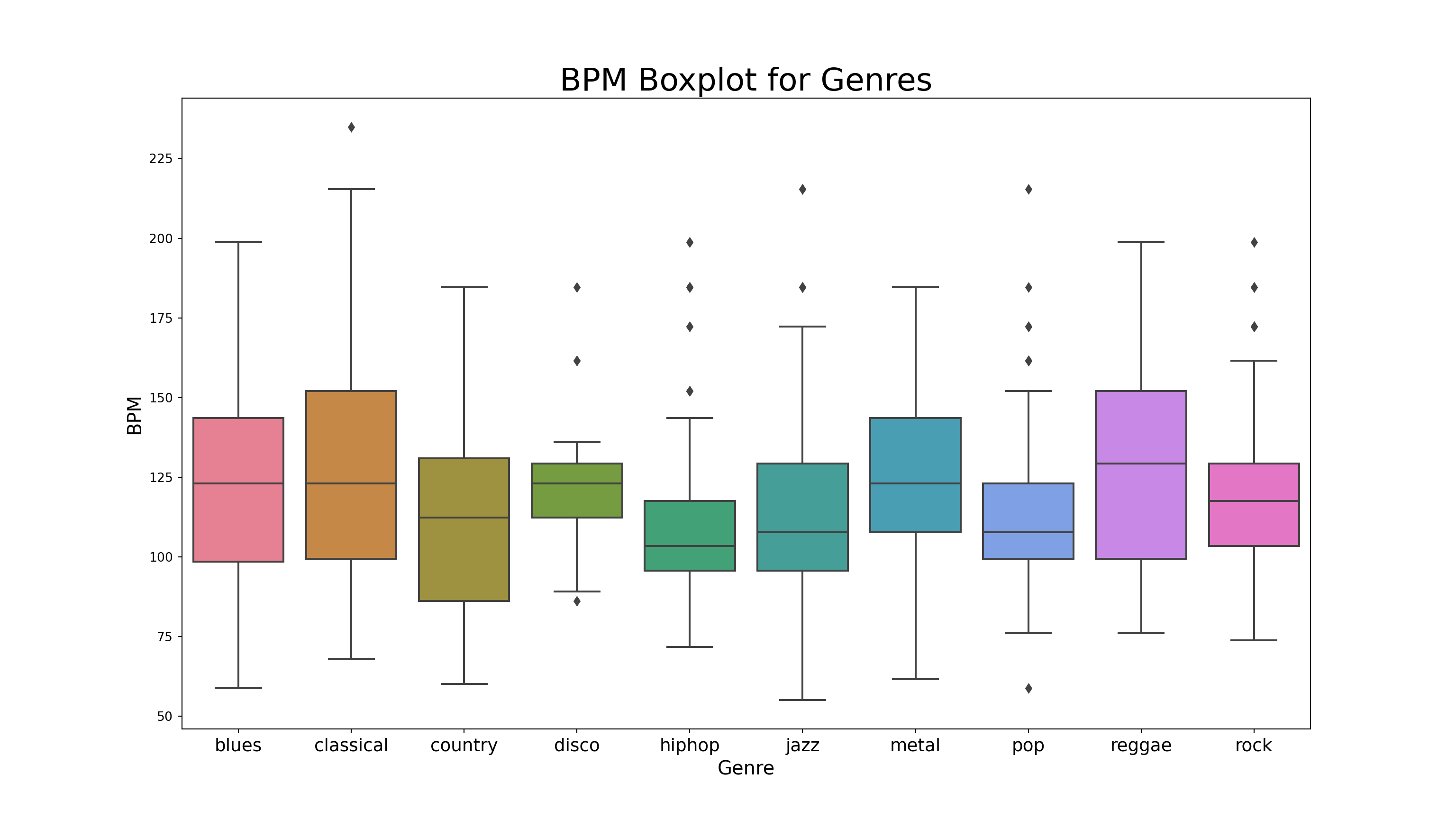

Principal Component Analysis

• For this part, we will conduct a principal component analysis (PCA) to visualize possible groups of genres and display its results with a scatter plot. We can see that a lot of songs have ambiguous genres; that is, it could be classified into more than one similar genres such as disco or hiphop based on the sound characteristics that we extract from them. There is also a song that is exclusively classified into a genre (reggae, for example).

Show code

from sklearn import preprocessing

data = data.iloc[0:, 1:]
y = data['label']
X = data.loc[:, data.columns != 'label']

#### NORMALIZE X ####
cols = X.columns
min_max_scaler = preprocessing.MinMaxScaler()
np_scaled = min_max_scaler.fit_transform(X)
X = pd.DataFrame(np_scaled, columns = cols)


#### PCA 2 COMPONENTS ####
from sklearn.decomposition import PCA

pca = PCA(n_components=2)
principalComponents = pca.fit_transform(X)
principalDf = pd.DataFrame(data = principalComponents, columns = ['principal component 1', 'principal component 2'])

# concatenate with target label
finalDf = pd.concat([principalDf, y], axis = 1)

pca.explained_variance_ratio_

# 44.93 variance explained

array([0.2439355 , 0.21781804])

Show code

plt.figure(figsize = (16, 9))

<Figure size 1600x900 with 0 Axes>

Show code

sns.scatterplot(x = "principal component 1", y = "principal component 2", data = finalDf, hue = "label", alpha = 0.7,
               s = 100);

plt.title('PCA on Genres', fontsize = 25)

Text(0.5, 1.0, 'PCA on Genres')

Show code

plt.xticks(fontsize = 14)

(array([-1.5, -1. , -0.5,  0. ,  0.5,  1. ,  1.5]), [Text(0, 0, ''), Text(0, 0, ''), Text(0, 0, ''), Text(0, 0, ''), Text(0, 0, ''), Text(0, 0, ''), Text(0, 0, '')])

Show code

plt.yticks(fontsize = 10);
plt.xlabel("Principal Component 1", fontsize = 15)

Text(0.5, 0, 'Principal Component 1')

Show code

plt.ylabel("Principal Component 2", fontsize = 15)

Text(0, 0.5, 'Principal Component 2')

Show code

plt.show()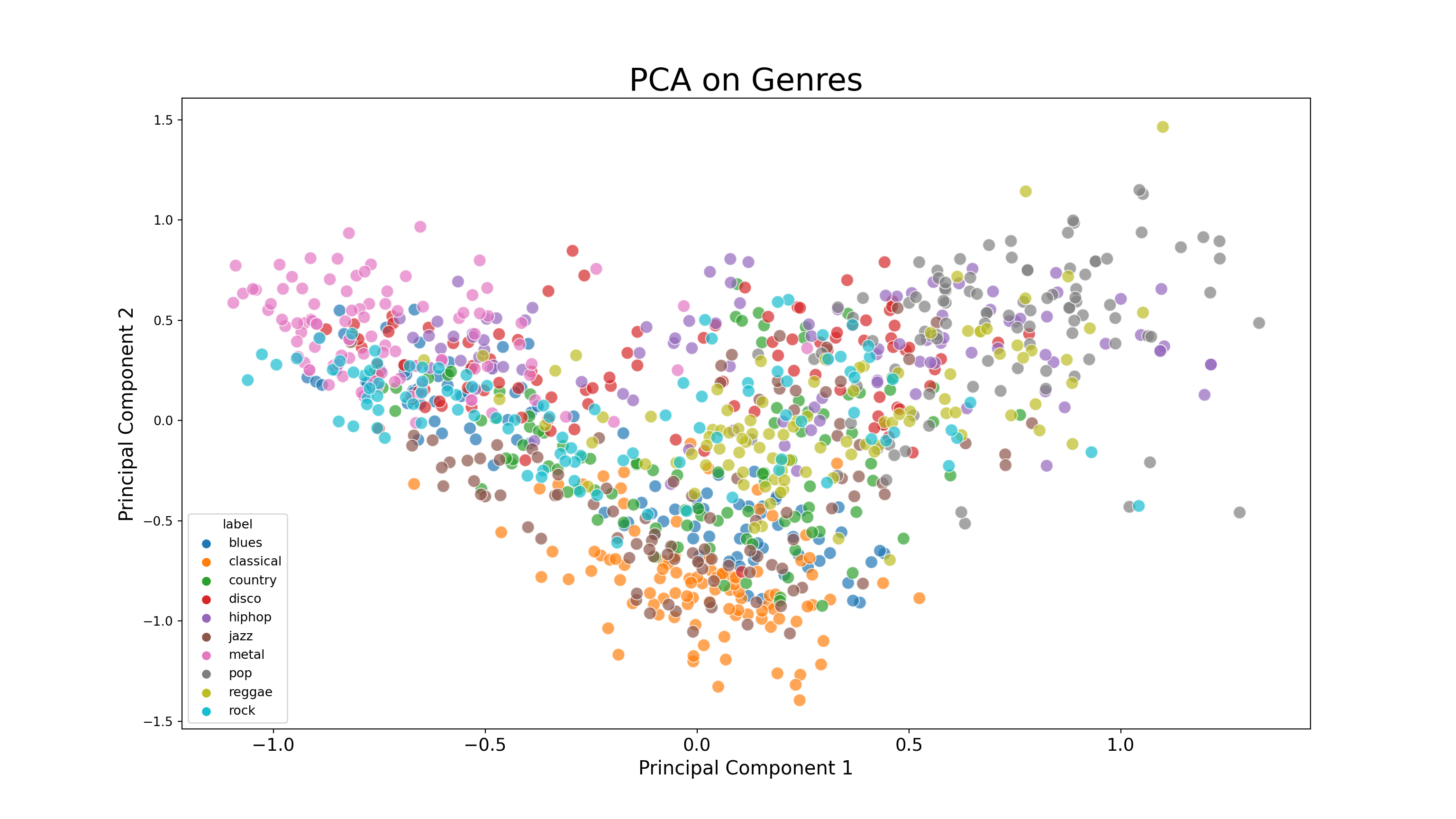

Machine Learning Classification

• Using features from features_3_sec.csv file, we can build a machine learning classification model that predicts genre of a new audio file. We will be loading a lot of machine learning models to see which model performs best.

Show code

from sklearn.naive_bayes import GaussianNB
from sklearn.linear_model import SGDClassifier, LogisticRegression
from sklearn.neighbors import KNeighborsClassifier
from sklearn.tree import DecisionTreeClassifier
from sklearn.ensemble import RandomForestClassifier
from sklearn.svm import SVC
from sklearn.neural_network import MLPClassifier
from xgboost import XGBClassifier, XGBRFClassifier
from xgboost import plot_tree, plot_importance

from sklearn.metrics import confusion_matrix, accuracy_score, roc_auc_score, roc_curve
from sklearn import preprocessing
from sklearn.model_selection import train_test_split
from sklearn.feature_selection import RFE

Reading in the Data

• We will read the data, split it into training and testing data sets, and create a function to assess accuracy of the models.

Show code

data = pd.read_csv('features_3_sec.csv')
data = data.iloc[0:, 1:] 
data.head()

   length  chroma_stft_mean  chroma_stft_var  ...  mfcc20_mean  mfcc20_var  label
0   66149          0.335406         0.091048  ...    -0.243027   43.771767  blues
1   66149          0.343065         0.086147  ...     5.784063   59.943081  blues
2   66149          0.346815         0.092243  ...     2.517375   33.105122  blues
3   66149          0.363639         0.086856  ...     3.630866   32.023678  blues
4   66149          0.335579         0.088129  ...     0.536961   29.146694  blues

[5 rows x 59 columns]

Features and Target variable

• Create features and target variable, as well as normalizing the data.

Show code

y = data['label'] # genre variable.
X = data.loc[:, data.columns != 'label'] #select all columns but not the labels

#### NORMALIZE X ####

# Normalize so everything is on the same scale. 

cols = X.columns
min_max_scaler = preprocessing.MinMaxScaler()
np_scaled = min_max_scaler.fit_transform(X)

# new data frame with the new scaled data. 
X = pd.DataFrame(np_scaled, columns = cols)

X_train, X_test, y_train, y_test = train_test_split(X, y, test_size=0.3, random_state=42)

Show code

#Creating a Predefined function to assess the accuracy of a model

def model_assess(model, title = "Default"):
    model.fit(X_train, y_train)
    preds = model.predict(X_test)
    #print(confusion_matrix(y_test, preds))
    print('Accuracy', title, ':', round(accuracy_score(y_test, preds), 5), '\n')

• Here, we will test 10 different machine learning models to see which model is most suitable to music classification task.

Show code

# Naive Bayes
nb = GaussianNB()
model_assess(nb, "Naive Bayes")

# Stochastic Gradient Descent

Accuracy Naive Bayes : 0.51952 

Show code

sgd = SGDClassifier(max_iter=5000, random_state=0)
model_assess(sgd, "Stochastic Gradient Descent")

# KNN

Accuracy Stochastic Gradient Descent : 0.65532 

Show code

knn = KNeighborsClassifier(n_neighbors=19)
model_assess(knn, "KNN")

# Decission trees

Accuracy KNN : 0.80581 

Show code

tree = DecisionTreeClassifier()
model_assess(tree, "Decission trees")

# Random Forest

Accuracy Decission trees : 0.6383 

Show code

rforest = RandomForestClassifier(n_estimators=1000, max_depth=10, random_state=0)
model_assess(rforest, "Random Forest")

# Support Vector Machine

Accuracy Random Forest : 0.81415 

Show code

svm = SVC(decision_function_shape="ovo")
model_assess(svm, "Support Vector Machine")

# Logistic Regression

Accuracy Support Vector Machine : 0.75409 

Show code

lg = LogisticRegression(random_state=0, solver='lbfgs', multi_class='multinomial')
model_assess(lg, "Logistic Regression")

# Neural Nets

Accuracy Logistic Regression : 0.6977 


C:\Users\tarid\AppData\Roaming\Python\Python38\site-packages\sklearn\linear_model\_logistic.py:762: ConvergenceWarning: lbfgs failed to converge (status=1):
STOP: TOTAL NO. of ITERATIONS REACHED LIMIT.

Increase the number of iterations (max_iter) or scale the data as shown in:
    https://scikit-learn.org/stable/modules/preprocessing.html
Please also refer to the documentation for alternative solver options:
    https://scikit-learn.org/stable/modules/linear_model.html#logistic-regression
  n_iter_i = _check_optimize_result(

Show code

nn = MLPClassifier(solver='lbfgs', alpha=1e-5, hidden_layer_sizes=(5000, 10), random_state=1)
model_assess(nn, "Neural Nets")

# Cross Gradient Booster

Accuracy Neural Nets : 0.67401 


C:\Users\tarid\AppData\Roaming\Python\Python38\site-packages\sklearn\neural_network\_multilayer_perceptron.py:471: ConvergenceWarning: lbfgs failed to converge (status=1):
STOP: TOTAL NO. of ITERATIONS REACHED LIMIT.

Increase the number of iterations (max_iter) or scale the data as shown in:
    https://scikit-learn.org/stable/modules/preprocessing.html
  self.n_iter_ = _check_optimize_result("lbfgs", opt_res, self.max_iter)

Show code

xgb = XGBClassifier(n_estimators=1000, learning_rate=0.05, eval_metric='mlogloss')
model_assess(xgb, "Cross Gradient Booster")

# Cross Gradient Booster (Random Forest)

Accuracy Cross Gradient Booster : 0.90224 


C:\Users\tarid\ANACON~1\lib\site-packages\xgboost\sklearn.py:1224: UserWarning: The use of label encoder in XGBClassifier is deprecated and will be removed in a future release. To remove this warning, do the following: 1) Pass option use_label_encoder=False when constructing XGBClassifier object; and 2) Encode your labels (y) as integers starting with 0, i.e. 0, 1, 2, ..., [num_class - 1].
  warnings.warn(label_encoder_deprecation_msg, UserWarning)

Show code

xgbrf = XGBRFClassifier(objective= 'multi:softmax', eval_metric='mlogloss')
model_assess(xgbrf, "Cross Gradient Booster (Random Forest)")

Accuracy Cross Gradient Booster (Random Forest) : 0.74575 

• The function Extreme Gradient Boosting (XGBoost) achieves the highest performance with 90% accuracy. We will be using this model to create the final prediction model and compute feature importance output along with its confusion matrix.

• Note that I have also included Multilayer Perception - a variant of Neural Networks model - into the list of candidate models as well. While neural networks may be known for its complexity, it does not mean that the model is a silver bullet for every machine learning task. This idea is derived from the No Free Lunch Theorem that implies that there is no single best algorithm.

Show code

#Final model
xgb = XGBClassifier(n_estimators=1000, learning_rate=0.05, eval_metric='mlogloss')
xgb.fit(X_train, y_train)

XGBClassifier(base_score=0.5, booster='gbtree', colsample_bylevel=1,
              colsample_bynode=1, colsample_bytree=1, enable_categorical=False,
              eval_metric='mlogloss', gamma=0, gpu_id=-1, importance_type=None,
              interaction_constraints='', learning_rate=0.05, max_delta_step=0,
              max_depth=6, min_child_weight=1, missing=nan,
              monotone_constraints='()', n_estimators=1000, n_jobs=8,
              num_parallel_tree=1, objective='multi:softprob', predictor='auto',
              random_state=0, reg_alpha=0, reg_lambda=1, scale_pos_weight=None,
              subsample=1, tree_method='exact', validate_parameters=1,
              verbosity=None)

Show code

preds = xgb.predict(X_test)

print('Accuracy', ':', round(accuracy_score(y_test, preds), 5), '\n')

# Confusion Matrix

Accuracy : 0.90224 

Show code

confusion_matr = confusion_matrix(y_test, preds) #normalize = 'true'
plt.figure(figsize = (16, 9))

<Figure size 1600x900 with 0 Axes>

Show code

sns.heatmap(confusion_matr, cmap="Blues", annot=True,
            xticklabels = ["blues", "classical", "country", "disco", "hiphop", "jazz", "metal", "pop", "reggae", "rock"],
           yticklabels=["blues", "classical", "country", "disco", "hiphop", "jazz", "metal", "pop", "reggae", "rock"]);
plt.show()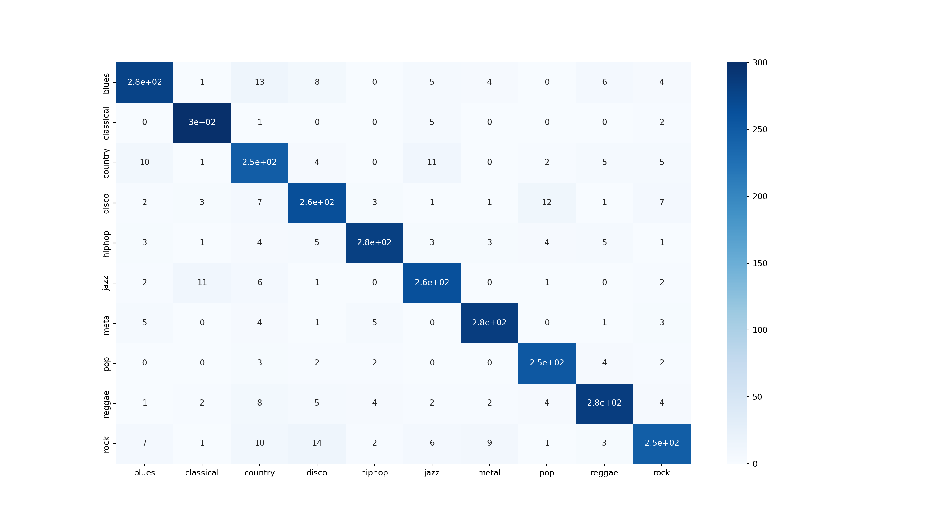

Feature Importance

• From the feature importance output, we can see that varianve and mean of the perceptual variable perceptr_var are the two most important variable in genre classification.

Show code

import eli5
from eli5.sklearn import PermutationImportance

perm = PermutationImportance(estimator=xgb, random_state=1)
perm.fit(X_test, y_test)

PermutationImportance(estimator=XGBClassifier(base_score=0.5, booster='gbtree',
                                              colsample_bylevel=1,
                                              colsample_bynode=1,
                                              colsample_bytree=1,
                                              enable_categorical=False,
                                              eval_metric='mlogloss', gamma=0,
                                              gpu_id=-1, importance_type=None,
                                              interaction_constraints='',
                                              learning_rate=0.05,
                                              max_delta_step=0, max_depth=6,
                                              min_child_weight=1, missing=nan,
                                              monotone_constraints='()',
                                              n_estimators=1000, n_jobs=8,
                                              num_parallel_tree=1,
                                              objective='multi:softprob',
                                              predictor='auto', random_state=0,
                                              reg_alpha=0, reg_lambda=1,
                                              scale_pos_weight=None,
                                              subsample=1, tree_method='exact',
                                              validate_parameters=1,
                                              verbosity=None),
                      random_state=1)

Show code

eli5.show_weights(estimator=perm, feature_names = X_test.columns.tolist())

<IPython.core.display.HTML object>

Music recommendation algorithm

• The music recommendation system assumes that the audience likes to listen to music of similar genres or similar characteristics. The system allows us to find the best similarity, ranked in descending order, from the bast match to the least best match with the cosine_similarity statistics.

Show code

# Libraries
import IPython.display as ipd
from sklearn.metrics.pairwise import cosine_similarity
from sklearn import preprocessing

# Read data
data = pd.read_csv('features_30_sec.csv', index_col='filename')

# Extract labels
labels = data[['label']]

# Drop labels from original dataframe
data = data.drop(columns=['length','label'])
data.head()

# Scale the data

                 chroma_stft_mean  chroma_stft_var  ...  mfcc20_mean  mfcc20_var
filename                                            ...                         
blues.00000.wav          0.350088         0.088757  ...     1.221291   46.936035
blues.00001.wav          0.340914         0.094980  ...     0.531217   45.786282
blues.00002.wav          0.363637         0.085275  ...    -2.231258   30.573025
blues.00003.wav          0.404785         0.093999  ...    -3.407448   31.949339
blues.00004.wav          0.308526         0.087841  ...   -11.703234   55.195160

[5 rows x 57 columns]

Show code

data_scaled=preprocessing.scale(data)
print('Scaled data type:', type(data_scaled))

Scaled data type: <class 'numpy.ndarray'>

Cosine Similarity

• We will calculate the pairwise cosine similarity for each combination of songs in the data. The closer the value is to “1”, the more similar the two songs can be.

Show code

# Cosine similarity
similarity = cosine_similarity(data_scaled)
print("Similarity shape:", similarity.shape)

# Convert into a dataframe and then set the row index and column names as labels

Similarity shape: (1000, 1000)

Show code

sim_df_labels = pd.DataFrame(similarity)
sim_df_names = sim_df_labels.set_index(labels.index)
sim_df_names.columns = labels.index

sim_df_names.head()

filename         blues.00000.wav  ...  rock.00099.wav
filename                          ...                
blues.00000.wav         1.000000  ...        0.304098
blues.00001.wav         0.049231  ...        0.311723
blues.00002.wav         0.589618  ...        0.321069
blues.00003.wav         0.284862  ...        0.183210
blues.00004.wav         0.025561  ...        0.061785

[5 rows x 1000 columns]

Song similarity scoring

• We will define a function find_similar_songs() to take the name of the song and return top 5 best matches for that song.

Show code

def find_similar_songs(name):
    # Find songs most similar to another song
    series = sim_df_names[name].sort_values(ascending = False)
    
    # Remove cosine similarity == 1 (songs will always have the best match with themselves)
    series = series.drop(name)
    
    # Display the 5 top matches 
    print("\n*******\nSimilar songs to ", name)
    print(series.head(5))

• Now let us try putting it to the test:

Show code

find_similar_songs('pop.00023.wav') 

*******
Similar songs to  pop.00023.wav
filename
pop.00075.wav    0.875235
pop.00089.wav    0.874246
pop.00088.wav    0.872443
pop.00091.wav    0.871975
pop.00024.wav    0.869849
Name: pop.00023.wav, dtype: float64

Show code

find_similar_songs('pop.00078.wav') 

*******
Similar songs to  pop.00078.wav
filename
pop.00088.wav       0.914322
hiphop.00077.wav    0.876289
pop.00089.wav       0.871822
pop.00074.wav       0.855630
pop.00023.wav       0.854349
Name: pop.00078.wav, dtype: float64

Show code

find_similar_songs('rock.00018.wav') 

*******
Similar songs to  rock.00018.wav
filename
rock.00017.wav     0.921997
metal.00028.wav    0.913790
metal.00058.wav    0.912421
rock.00016.wav     0.912421
rock.00026.wav     0.910113
Name: rock.00018.wav, dtype: float64

Show code

find_similar_songs('metal.00002.wav') 

*******
Similar songs to  metal.00002.wav
filename
metal.00028.wav    0.904367
metal.00059.wav    0.896096
rock.00018.wav     0.891910
rock.00017.wav     0.886526
rock.00016.wav     0.867508
Name: metal.00002.wav, dtype: float64

• The output above shows similarity score for the sampled song. For example, the top three similar songs to pop.00023 - Britney Spears - “I’m so curious (2009 remaster)” are pop.00075, pop.00089, and pop.00088 respectively.

• The algorithm can also recommend similar songs from other genres as well, for example, metal.00002 - Iron Maiden “Flight of Icarus”has similar songs in both metal and rock genre. The same thing also applies to rock.00018 - Queens - “Another One Bites The Dust” that has similar songs in both metal and rock genre as well.

Concluding note

• It is interesting in how we are able to process audio data into numbers or images. The application of music recognition algorithm could be highly beneficial to entertainment industry in meeting the needs of consumer market. Researchers can also apply algorithm of this nature to extract characteristics that may be useful to their variable of interest such as attention or mental concentration.

• One thing worth noting is, I am not a music expert, though I would love to practice piano at some point. The algorithm that I used is just one way of classifying musics into genres with the available information (e.g., tempo, harmonic wave). Domain expertise is important in data work regardless of your skill in data science. That is why it is crucial to consult with experts of the subject matter (i.e., musician) to make the most out of the insight we gained from this data. This also applies to other area such as testing as well. I can do the math and the programming, but I don’t know much about students or English testing. This is where domain experts come into play. I just want to emphasize the importance of collaboration between fields to ensure the best results for the collective good.

• Due to the nature of my field (education), it is unlikely that I will have much chance to work with audio data, but this practice is still valuable regardless. The model_assess function that I used can be applied to any machine learning work that requires the use of several models to find the most suitable algorithm for the task. The cosine_similarity statistics is also useful to recommendation system of any products such as textbooks or novels. Anyway, it was a good practice, and I had fun nonetheless. As always, thank you very much for your read! I hope you have a good day wherever you are!