Examining the Big 5 personality Dataset with factor analysis

For this entry, I will be examining the Big 5 personality Inventory data set with Exploratory Data Analysis to identify potential structures of personality trait and verify them with Confirmatory Factor Analysis.

(8 min read)

Introduction

• The concept of Big 5 personality traits represents tendency of individuals to possess five personality characteristics of extraversion, agreeableness, openness, conscientiousness, and neuroticism (Neal et al., 2012).

• Here, we will examine the data set with Exploratory Data Analysis (EFA) to see if we can identify any other structures aside from the original five groups as indicated by the concept of big 5 personality traits; then, we will verify those structures with Confirmatory Factor Analysis (CFA) to assess and compare their statistical characteristic (i.e., model fit).

• We will begin by loading essential packages for data preprocessing and statistical modeling as indicated below.

Show code

library(parameters) #for parameter processing
library(tidymodels) #for data splitting
library(tidyverse) #toolbox for R
library(psych) #for descriptive statistics and the data set
library(ggcorrplot) #for correlation matrix
library(see) #add-on for ggplot2
library(lavaan) #for SEM
library(performance) #assessment of Regression Models Performance
library(semPlot) #to plot path model for CFA
library(dlookr) #missing data diagnosis
library(mice) #missing data imputation

Dataset

• The data set we use is a built-in data set from psych package, which was collected in the United States as a part of the Synthetic Aperture Personality Assessment (SAPA) project (Revelle et al., 2010). There are 2800 observations and 25 variables of all 5 personality traits.

• We will begin by loading in the data set and check for its missing value.

Show code

# Load the data
data <- psych::bfi[, 1:25]

head(data)

      A1 A2 A3 A4 A5 C1 C2 C3 C4 C5 E1 E2 E3 E4 E5 N1 N2 N3 N4 N5 O1
61617  2  4  3  4  4  2  3  3  4  4  3  3  3  4  4  3  4  2  2  3  3
61618  2  4  5  2  5  5  4  4  3  4  1  1  6  4  3  3  3  3  5  5  4
61620  5  4  5  4  4  4  5  4  2  5  2  4  4  4  5  4  5  4  2  3  4
61621  4  4  6  5  5  4  4  3  5  5  5  3  4  4  4  2  5  2  4  1  3
61622  2  3  3  4  5  4  4  5  3  2  2  2  5  4  5  2  3  4  4  3  3
61623  6  6  5  6  5  6  6  6  1  3  2  1  6  5  6  3  5  2  2  3  4
      O2 O3 O4 O5
61617  6  3  4  3
61618  2  4  3  3
61620  2  5  5  2
61621  3  4  3  5
61622  3  4  3  3
61623  3  5  6  1

Show code

#diagnose for missing value
dlookr::diagnose(data)

# A tibble: 25 x 6
   variables types   missing_count missing_percent unique_count
   <chr>     <chr>           <int>           <dbl>        <int>
 1 A1        integer            16           0.571            7
 2 A2        integer            27           0.964            7
 3 A3        integer            26           0.929            7
 4 A4        integer            19           0.679            7
 5 A5        integer            16           0.571            7
 6 C1        integer            21           0.75             7
 7 C2        integer            24           0.857            7
 8 C3        integer            20           0.714            7
 9 C4        integer            26           0.929            7
10 C5        integer            16           0.571            7
# ... with 15 more rows, and 1 more variable: unique_rate <dbl>

Show code

visdat::vis_miss(data, sort_miss = FALSE)

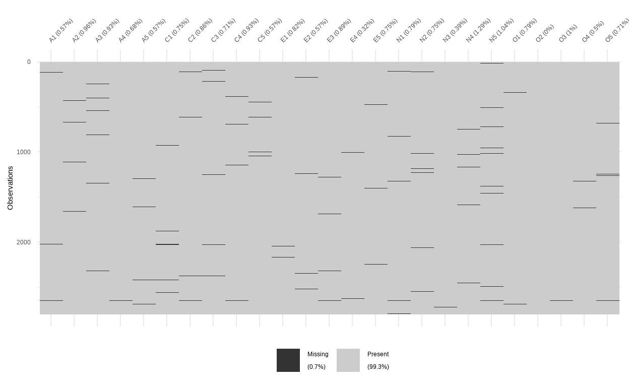
• There are some degree of missingness in the dataset as indicated by the missingness map. For good measure, we will impute it with the predictive mean matchmaking method by the mice package.

Data preprocessing

Show code

#imputation
mice_model <- mice(data, method='pmm', seed = 123)

 iter imp variable
  1   1  A1  A2  A3  A4  A5  C1  C2  C3  C4  C5  E1  E2  E3  E4  E5  N1  N2  N3  N4  N5  O1  O3  O4  O5
  1   2  A1  A2  A3  A4  A5  C1  C2  C3  C4  C5  E1  E2  E3  E4  E5  N1  N2  N3  N4  N5  O1  O3  O4  O5
  1   3  A1  A2  A3  A4  A5  C1  C2  C3  C4  C5  E1  E2  E3  E4  E5  N1  N2  N3  N4  N5  O1  O3  O4  O5
  1   4  A1  A2  A3  A4  A5  C1  C2  C3  C4  C5  E1  E2  E3  E4  E5  N1  N2  N3  N4  N5  O1  O3  O4  O5
  1   5  A1  A2  A3  A4  A5  C1  C2  C3  C4  C5  E1  E2  E3  E4  E5  N1  N2  N3  N4  N5  O1  O3  O4  O5
  2   1  A1  A2  A3  A4  A5  C1  C2  C3  C4  C5  E1  E2  E3  E4  E5  N1  N2  N3  N4  N5  O1  O3  O4  O5
  2   2  A1  A2  A3  A4  A5  C1  C2  C3  C4  C5  E1  E2  E3  E4  E5  N1  N2  N3  N4  N5  O1  O3  O4  O5
  2   3  A1  A2  A3  A4  A5  C1  C2  C3  C4  C5  E1  E2  E3  E4  E5  N1  N2  N3  N4  N5  O1  O3  O4  O5
  2   4  A1  A2  A3  A4  A5  C1  C2  C3  C4  C5  E1  E2  E3  E4  E5  N1  N2  N3  N4  N5  O1  O3  O4  O5
  2   5  A1  A2  A3  A4  A5  C1  C2  C3  C4  C5  E1  E2  E3  E4  E5  N1  N2  N3  N4  N5  O1  O3  O4  O5
  3   1  A1  A2  A3  A4  A5  C1  C2  C3  C4  C5  E1  E2  E3  E4  E5  N1  N2  N3  N4  N5  O1  O3  O4  O5
  3   2  A1  A2  A3  A4  A5  C1  C2  C3  C4  C5  E1  E2  E3  E4  E5  N1  N2  N3  N4  N5  O1  O3  O4  O5
  3   3  A1  A2  A3  A4  A5  C1  C2  C3  C4  C5  E1  E2  E3  E4  E5  N1  N2  N3  N4  N5  O1  O3  O4  O5
  3   4  A1  A2  A3  A4  A5  C1  C2  C3  C4  C5  E1  E2  E3  E4  E5  N1  N2  N3  N4  N5  O1  O3  O4  O5
  3   5  A1  A2  A3  A4  A5  C1  C2  C3  C4  C5  E1  E2  E3  E4  E5  N1  N2  N3  N4  N5  O1  O3  O4  O5
  4   1  A1  A2  A3  A4  A5  C1  C2  C3  C4  C5  E1  E2  E3  E4  E5  N1  N2  N3  N4  N5  O1  O3  O4  O5
  4   2  A1  A2  A3  A4  A5  C1  C2  C3  C4  C5  E1  E2  E3  E4  E5  N1  N2  N3  N4  N5  O1  O3  O4  O5
  4   3  A1  A2  A3  A4  A5  C1  C2  C3  C4  C5  E1  E2  E3  E4  E5  N1  N2  N3  N4  N5  O1  O3  O4  O5
  4   4  A1  A2  A3  A4  A5  C1  C2  C3  C4  C5  E1  E2  E3  E4  E5  N1  N2  N3  N4  N5  O1  O3  O4  O5
  4   5  A1  A2  A3  A4  A5  C1  C2  C3  C4  C5  E1  E2  E3  E4  E5  N1  N2  N3  N4  N5  O1  O3  O4  O5
  5   1  A1  A2  A3  A4  A5  C1  C2  C3  C4  C5  E1  E2  E3  E4  E5  N1  N2  N3  N4  N5  O1  O3  O4  O5
  5   2  A1  A2  A3  A4  A5  C1  C2  C3  C4  C5  E1  E2  E3  E4  E5  N1  N2  N3  N4  N5  O1  O3  O4  O5
  5   3  A1  A2  A3  A4  A5  C1  C2  C3  C4  C5  E1  E2  E3  E4  E5  N1  N2  N3  N4  N5  O1  O3  O4  O5
  5   4  A1  A2  A3  A4  A5  C1  C2  C3  C4  C5  E1  E2  E3  E4  E5  N1  N2  N3  N4  N5  O1  O3  O4  O5
  5   5  A1  A2  A3  A4  A5  C1  C2  C3  C4  C5  E1  E2  E3  E4  E5  N1  N2  N3  N4  N5  O1  O3  O4  O5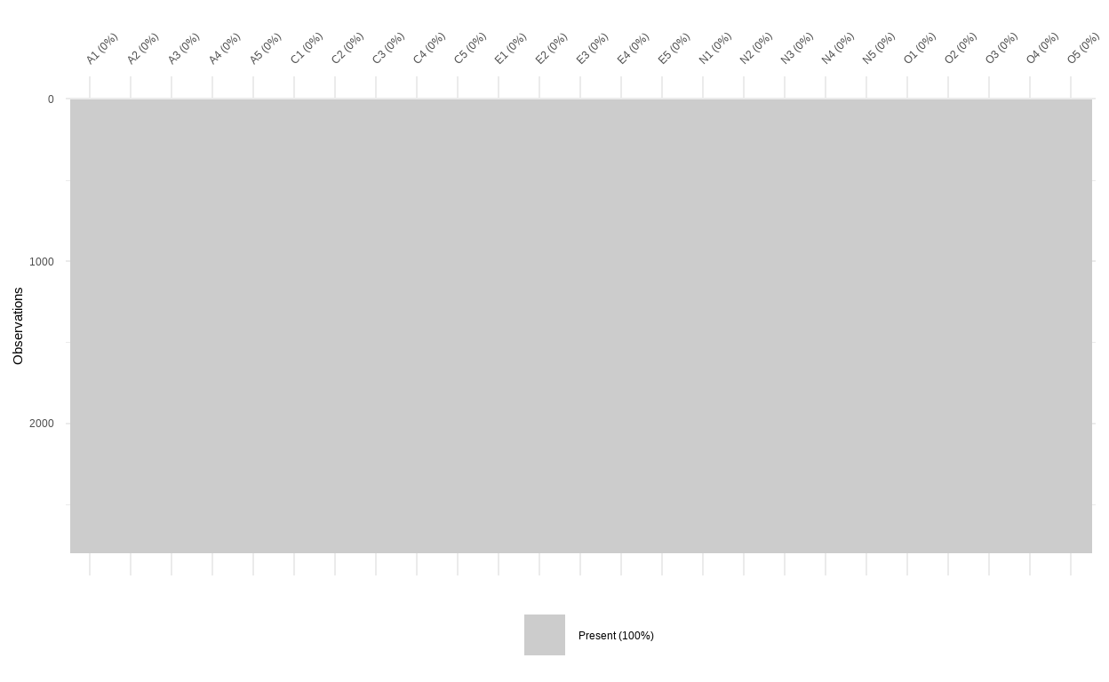

Show code

data_complete <- complete(mice_model)

visdat::vis_miss(data_complete, sort_miss = FALSE)

• There is no missing value present in the dataset after the imputation. We can proceed with factor structure checking to assess whether the dataset is appropriate for factor analysis with check_factorstructure(). Two existing methods are the Bartlett’s Test of Sphericity and the Kaiser, Meyer, Olkin (KMO) Measure of Sampling Adequacy (MSA).

• The former tests whether a matrix is significantly different from an identity matrix. This statistical test for the presence of correlations among variables, providing the statistical probability that the correlation matrix has significant correlations among at least some of variables. As for factor analysis to work, some relationships between variables are needed, thus, a significant Bartlett’s test of sphericity is required to be significant.

• The latter method, ranging from 0 to 1, indicates the degree to which each variable in the dataset is predicted without error by the other variables. A value of 0 indicates that the sum of partial correlations is large relative to the sum correlations, indicating factor analysis is likely to be inappropriate. A KMO value close to 1 indicates that the sum of partial correlations is not large relative to the sum of correlations and so factor analysis should yield distinct and reliable factors.

Show code

#check for factor structure
check_factorstructure(data_complete)

# Is the data suitable for Factor Analysis?

  - KMO: The Kaiser, Meyer, Olkin (KMO) measure of sampling adequacy suggests that data seems appropriate for factor analysis (KMO = 0.84).
  - Sphericity: Bartlett's test of sphericity suggests that there is sufficient significant correlation in the data for factor analysis (Chisq(300) = 20158.27, p < .001).

• The Barlett’s test suggested that there is sufficient significant correlation in the data for factor analysis. Speaking of correlation, let us generate a correlation matrix to check for relationship between variables in the dataset as well.

Show code

variables.to.use<-c("A1", "A2", "A3", "A4", "A5",
                    "C1", "C2", "C3", "C4", "C5",
                    "E1", "E2", "E3", "E4", "E5",
                    "N1", "N2", "N3", "N4", "N5",
                    "O1", "O2", "O3", "O4", "O5")

data.corr<-cor(data_complete[variables.to.use],
                 method = "pearson",
                 use='all.obs')
ggcorrplot(data.corr,
           p.mat=cor_pmat(data_complete[variables.to.use]),
           hc.order=TRUE, 
           type='lower',
           color=c('red3', 'white', 'green3'),
           outline.color = 'darkgoldenrod1', 
           lab=FALSE, #omit the correlation coefficient
           legend.title='Correlation',
           pch=4, 
           pch.cex=4, #size of the cross mark for non-significant indicator
           lab_size=6)+ 
  labs(title="Correlation Matrix")+
  theme(plot.title=element_text(face='bold',size=14,hjust=0.5,colour="darkred"))+
  theme(legend.position=c(0.10,0.80), legend.box.just = "bottom")

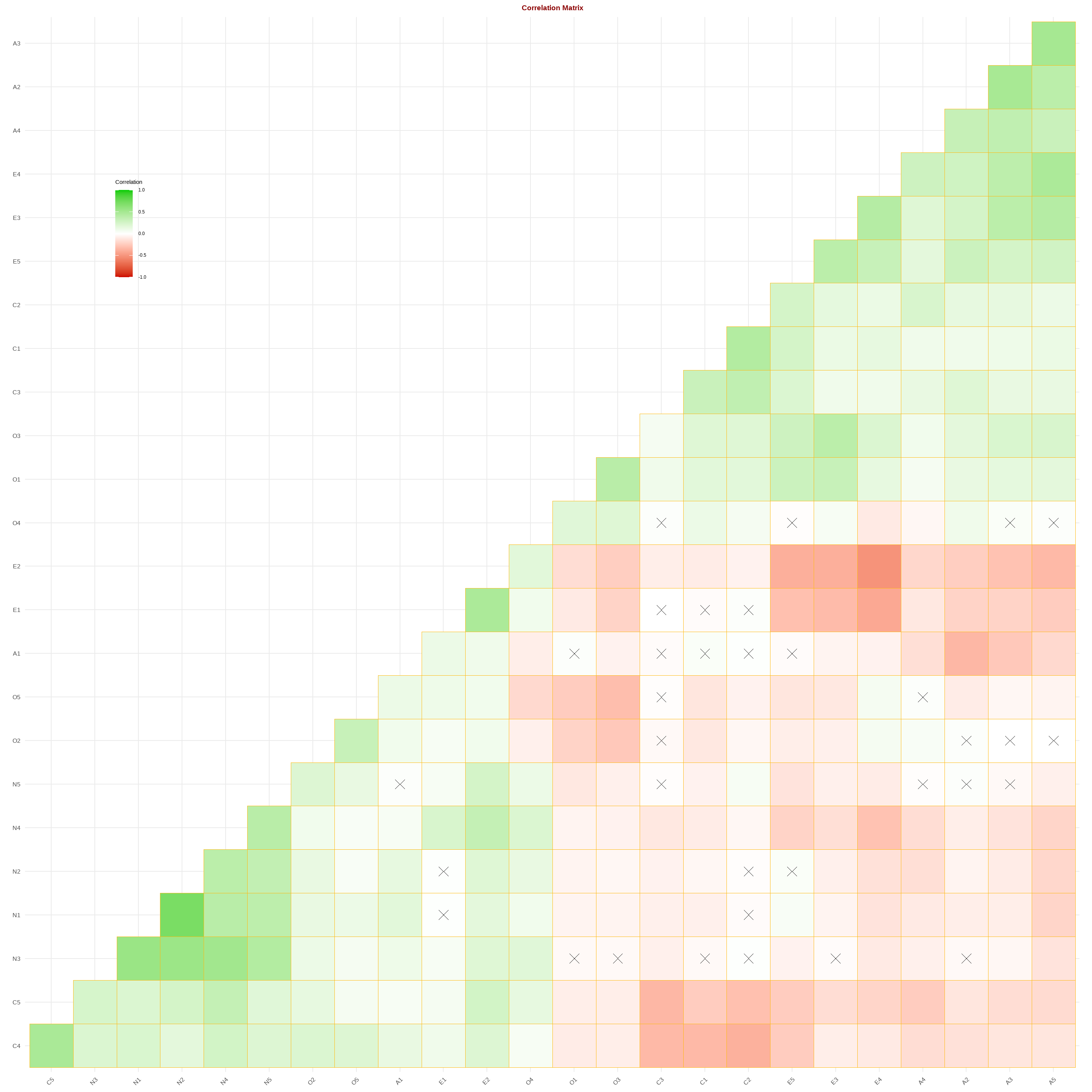
• The green panel indicates positive relationships while the red panel indicates negative relationship. The cross symbol suggests that the relationship between two variables is not statistically significant.

• Next, we would need to split the dataset into two to perform EFA and CFA, so that we can make sure to test the model on an unseen set of data.

Show code

# Establish two sets of indices to split the dataset
N <- nrow(data_complete)
indices <- seq(1, N)
indices_EFA <- sample(indices, floor((.5*N)))
indices_CFA <- indices[!(indices %in% indices_EFA)]

# Use those indices to split the dataset into halves for your EFA and CFA
bfi_EFA <- data_complete[indices_EFA, ]
bfi_CFA <- data_complete[indices_CFA, ]

Show code

check_factorstructure(bfi_EFA)

# Is the data suitable for Factor Analysis?

  - KMO: The Kaiser, Meyer, Olkin (KMO) measure of sampling adequacy suggests that data seems appropriate for factor analysis (KMO = 0.84).
  - Sphericity: Bartlett's test of sphericity suggests that there is sufficient significant correlation in the data for factor analysis (Chisq(300) = 10244.89, p < .001).

Show code

check_factorstructure(bfi_CFA)

# Is the data suitable for Factor Analysis?

  - KMO: The Kaiser, Meyer, Olkin (KMO) measure of sampling adequacy suggests that data seems appropriate for factor analysis (KMO = 0.84).
  - Sphericity: Bartlett's test of sphericity suggests that there is sufficient significant correlation in the data for factor analysis (Chisq(300) = 10210.30, p < .001).

• The two datasets that we splitted are appropriate for factor analysis, so we can proceed with EFA as the first analysis

Exploratory Factor Analysis

• Exploratory Factor Analysis is a statistical technique in social science to explain the variance between several measured variables as a smaller set of latent variables. EFA is often used to consolidate survey data by revealing the groupings (factors) that underly individual questions.

• An EFA provides information on each item’s relationship to a single factor that is hypothesized to be represented by each of the items. EFA results give you basic information about how well items relate to that hypothesized construct.

• The common application of EFA is to investigate relationships between observed variable and latent variables (factor) such as measurement piloting.

Scree plot

• To empirically determine the dimensionality of your data, a common strategy is to examine the eigenvalues and scree plot.

• The scree plot is a visual representation of eigenvalues that determines potential dimensionality of the dataset. Eigenvalues can be generated from a principal component analysis or a factor analysis, and the scree() function calculates and plots both by default. Since eigen() finds eigenvalues via principal components analysis, we will use factors = FALSE so our scree plot will only display the values corresponding to those results.

Show code

# Calculate the correlation matrix first
bfi_EFA_cor <- cor(bfi_EFA, use = "pairwise.complete.obs") 

# Then use that correlation matrix to calculate eigenvalues
eigenvals <- eigen(bfi_EFA_cor)

# Look at the eigenvalues returned
eigenvals$values

 [1] 5.1697200 2.6134230 2.1562029 1.7907326 1.6067099 1.0566407
 [7] 0.8427603 0.7962665 0.7482662 0.7263301 0.6985177 0.6640562
[13] 0.6544223 0.5997338 0.5573358 0.5424657 0.5117708 0.4961194
[19] 0.4602673 0.4487993 0.4259742 0.4020084 0.3868776 0.3675815
[25] 0.2770178

Show code

# Then use the correlation matrix to create the scree plot

scree(bfi_EFA_cor, factors = FALSE)

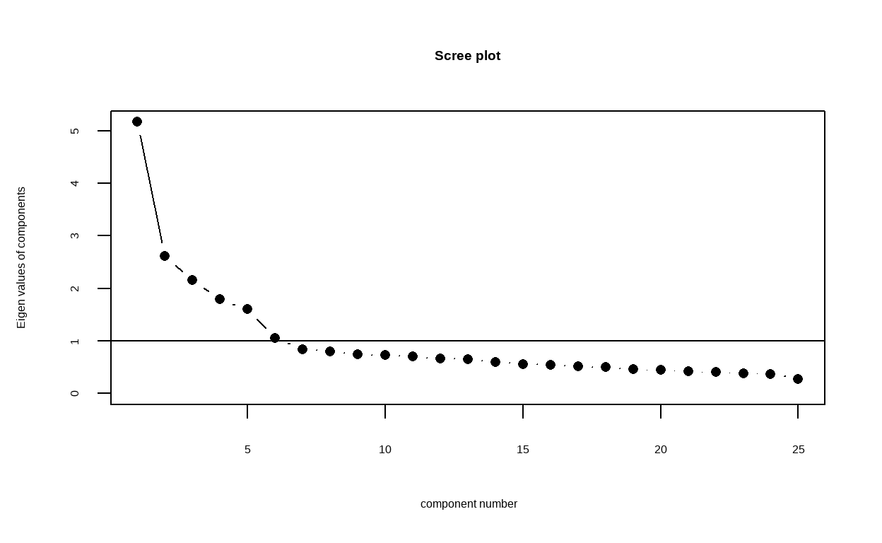
• From the above plot, The point where the slope of the curve is clearly leveling off (the “elbow) indicates that the number of factors that should be retained. For this case, the plot indicated that six factors should be retained.

• However, the dataset we use is for Big 5 personality traits with 5 factors, so we can investigate both 5 and 6 factors model to compare them both.

Fit EFA models

• We can initially explore the factor structure of 5 groups first as intended by the big 5 personality theory.

Show code

# Fit an EFA
efa <- psych::fa(data, nfactors = 5) %>% 
  model_parameters(sort = TRUE, threshold = "max")

efa

# Rotated loadings from Factor Analysis (oblimin-rotation)

Variable | MR2  |  MR1  |  MR3  |  MR5  |  MR4  | Complexity | Uniqueness
-------------------------------------------------------------------------
N1       | 0.81 |       |       |       |       |    1.08    |    0.35   
N2       | 0.78 |       |       |       |       |    1.04    |    0.40   
N3       | 0.71 |       |       |       |       |    1.07    |    0.45   
N5       | 0.49 |       |       |       |       |    1.96    |    0.65   
N4       | 0.47 |       |       |       |       |    2.27    |    0.51   
E2       |      | -0.68 |       |       |       |    1.07    |    0.46   
E4       |      | 0.59  |       |       |       |    1.49    |    0.47   
E1       |      | -0.56 |       |       |       |    1.21    |    0.65   
E5       |      | 0.42  |       |       |       |    2.60    |    0.60   
E3       |      | 0.42  |       |       |       |    2.55    |    0.56   
C2       |      |       | 0.67  |       |       |    1.17    |    0.55   
C4       |      |       | -0.61 |       |       |    1.18    |    0.55   
C3       |      |       | 0.57  |       |       |    1.11    |    0.68   
C5       |      |       | -0.55 |       |       |    1.44    |    0.57   
C1       |      |       | 0.55  |       |       |    1.19    |    0.67   
A3       |      |       |       | 0.66  |       |    1.07    |    0.48   
A2       |      |       |       | 0.64  |       |    1.04    |    0.55   
A5       |      |       |       | 0.53  |       |    1.49    |    0.54   
A4       |      |       |       | 0.43  |       |    1.74    |    0.72   
A1       |      |       |       | -0.41 |       |    1.97    |    0.81   
O3       |      |       |       |       | 0.61  |    1.17    |    0.54   
O5       |      |       |       |       | -0.54 |    1.21    |    0.70   
O1       |      |       |       |       | 0.51  |    1.13    |    0.69   
O2       |      |       |       |       | -0.46 |    1.75    |    0.74   
O4       |      |       |       |       | 0.37  |    2.69    |    0.75   

The 5 latent factors (oblimin rotation) accounted for 41.48% of the total variance of the original data (MR2 = 10.28%, MR1 = 8.80%, MR3 = 8.12%, MR5 = 7.94%, MR4 = 6.34%).

Show code

summary(efa)

# (Explained) Variance of Components

Parameter                       |   MR2 |   MR1 |   MR3 |   MR5 |   MR4
-----------------------------------------------------------------------
Eigenvalues                     | 4.493 | 2.249 | 1.505 | 1.188 | 0.934
Variance Explained              | 0.103 | 0.088 | 0.081 | 0.079 | 0.063
Variance Explained (Cumulative) | 0.103 | 0.191 | 0.272 | 0.351 | 0.415
Variance Explained (Proportion) | 0.248 | 0.212 | 0.196 | 0.191 | 0.153

• As we can see, the 25 items nicely spread on the 5 latent factors as the theory suggests. Based on this model, we can now predict back the scores for each individual for these new variables:

Show code

predict_result <- predict(efa, names = c("Neuroticism", "Conscientiousness", "Extraversion", "Agreeableness", "Opennness"))

head(predict_result)

  Neuroticism Conscientiousness Extraversion Agreeableness  Opennness
1 -0.21410935        0.06924675  -1.33208860   -0.85364725 -1.5809244
2  0.15008464        0.48139729  -0.59950262   -0.08478873 -0.1876070
3  0.62827949        0.10964162  -0.04800816   -0.55616873  0.2502735
4 -0.09425827        0.03836489  -1.05089539   -0.10394941 -1.1000032
5 -0.16368420        0.44253657  -0.10519669   -0.71857460 -0.6612203
6  0.18984314        1.08439177   1.40730835    0.39278790  0.6222356

How many factors should we retain?

• When running a factor analysis (FA), one often needs to specify how many components (or latent variables) to retain or to extract. This decision is often supported by some statistical indices and procedures aiming at finding the optimal number of factors, e.g., scree plot from (scree()).

• Interestingly, a huge amount of methods exist to statistically address this issue. These methods can sometimes contradict with each other in terms of retained factor. As a result, seeking the number that is supported by most methods is a reasonable compromise.

The Method Agreement procedure

• The Method Agreement procedure, first implemented in the psycho package, proposes to rely on the consensus of methods, rather than on one method in particular. This procedure can be used through the n_factors() by providing a dataframe, and the function will run a large number of routines and return the optimal number of factors based on the higher consensus.

Show code

n_factor <- parameters::n_factors(data_complete)

n_factor

# Method Agreement Procedure:

The choice of 6 dimensions is supported by 4 (21.05%) methods out of 19 (Optimal coordinates, Parallel analysis, Kaiser criterion, Scree (SE)).

Show code

as.data.frame(n_factor)

   n_Factors              Method              Family
1          1 Acceleration factor               Scree
2          3                 CNG                 CNG
3          4                beta Multiple_regression
4          4          Scree (R2)            Scree_SE
5          4    VSS complexity 1                 VSS
6          5    VSS complexity 2                 VSS
7          5       Velicer's MAP        Velicers_MAP
8          6 Optimal coordinates               Scree
9          6   Parallel analysis               Scree
10         6    Kaiser criterion               Scree
11         6          Scree (SE)            Scree_SE
12         7                   t Multiple_regression
13         7                   p Multiple_regression
14         8                 BIC                 BIC
15        12      BIC (adjusted)                 BIC
16        22             Bentler             Bentler
17        24            Bartlett             Barlett
18        24            Anderson             Barlett
19        24              Lawley             Barlett

• For more details, a summary table can be obtained

Show code

summary(n_factor)

   n_Factors n_Methods
1          1         1
2          3         1
3          4         3
4          5         2
5          6         4
6          7         2
7          8         1
8         12         1
9         22         1
10        24         3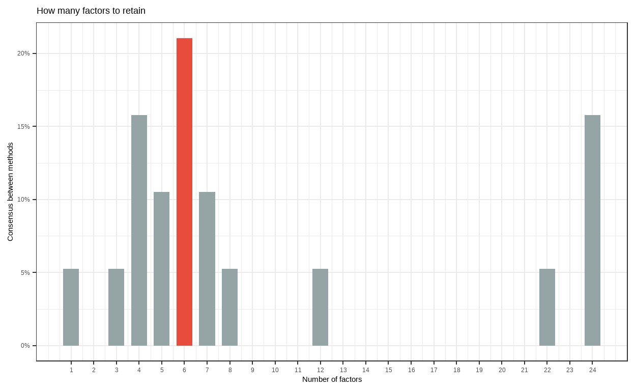

Show code

plot(n_factor) + theme_bw()

• Interestingly, most methods also suggest six factors from the model, which is consistent with the HEXACO model of personalities that is similar with the Big 5 personality theory.

Confirmatory Factor Analysis

• We’ve seen above that while an EFA with 5 latent variables works great on our dataset, a structure with 6 latent factors may be statistically viable as well. This topic can be statistically tested with a CFA to bridge factor analysis with Structural Equation Modelling (SEM).

• However, in order to do that cleanly, EFA should be independent from CFA in the sense that the factor structure should be explored on a training set, and then tested (or “confirmed”) on a test set.

Train test split

• The data can be easily split into two sets with the initial_split() of the tidymodel package, through which we will use 70% of the sample as the training and the rest as the test dataset.

Show code

set.seed(999)

# Put 3/4 of the data into the training set 
data_split <- initial_split(bfi_CFA, prop = 0.7)

# Create data frames for the two sets:
training <- training(data_split) #3/4
test  <- testing(data_split)  #1/4

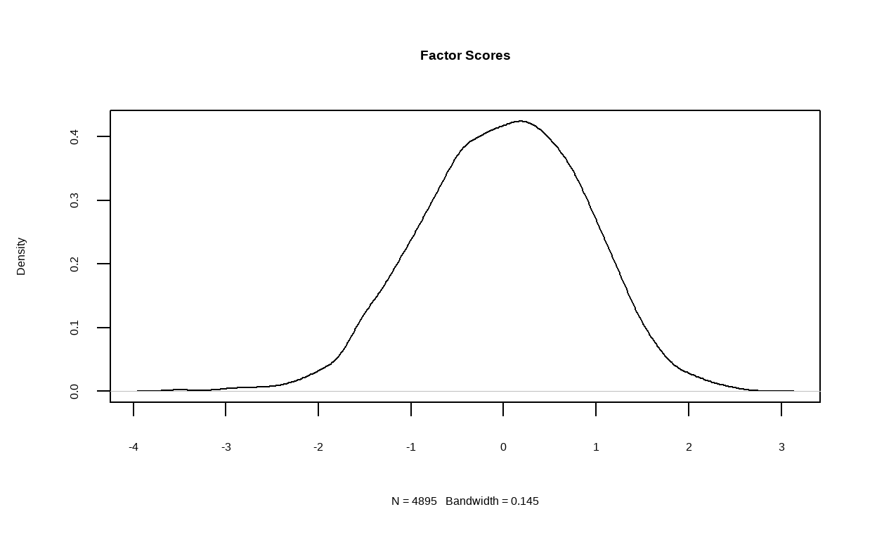
Create CFA structures out of EFA models

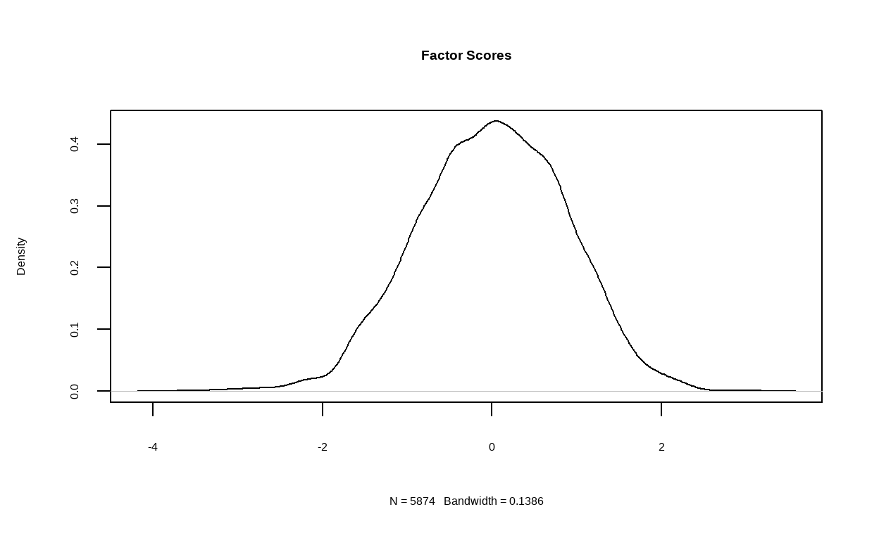
• In the next step, we will run two EFA models on the training set and specifying 5 and 6 latent factors respectively. We will also request for path diagram of the models as well as their density plot of factor score.

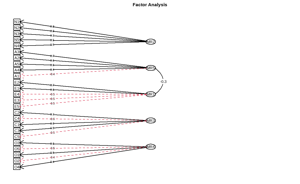
• First, we will examine structure of the 5 factors model.

Show code

structure_big5 <- psych::fa(training, nfactors = 5)
fa.diagram(structure_big5)

Show code

plot(density(structure_big5$scores, na.rm = TRUE), 
     main = "Factor Scores")

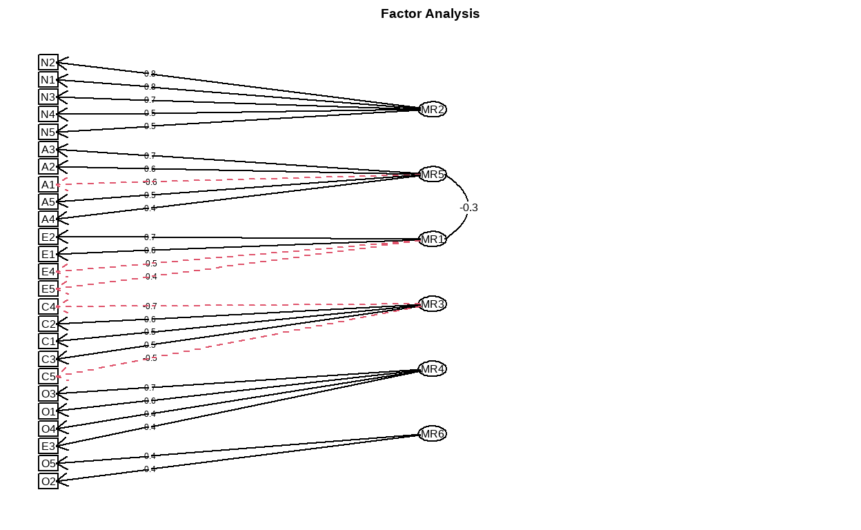
• Then, for the structure of the 6 factors model.

Show code

structure_big6 <- psych::fa(training, nfactors = 6) 
fa.diagram(structure_big6)

Show code

plot(density(structure_big6$scores, na.rm = TRUE), 
     main = "Factor Scores")

• We will then transform both EFA models into lavaan syntax to perform CFA.

Show code

#Converting EFA into a lavaan-ready syntax
cfa_big5 <- efa_to_cfa(structure_big5)

#Investigate how the model looks
cfa_big5

# Latent variables
MR2 =~ N1 + N2 + N3 + N4 + N5
MR5 =~ A1 + A2 + A3 + A4 + A5
MR1 =~ E1 + E2 + E3 + E4 + E5
MR3 =~ C1 + C2 + C3 + C4 + C5
MR4 =~ O1 + O2 + O3 + O4 + O5

Show code

cfa_big6 <- efa_to_cfa(structure_big6)
cfa_big6

# Latent variables
MR2 =~ N1 + N2 + N3 + N4 + N5
MR5 =~ A1 + A2 + A3 + A4 + A5
MR1 =~ E1 + E2 + E4 + E5
MR3 =~ C1 + C2 + C3 + C4 + C5
MR4 =~ E3 + O1 + O3 + O4
MR6 =~ O2 + O5

Fit and Compare models

• Next, we will fit both models with lavaan package before requesting for model fit measure with fitmeasures. We can also compare both models head-to-head with compare_performance.

Show code

model_big5 <- lavaan::cfa(cfa_big5, data = test)
model_big6 <- lavaan::cfa(cfa_big6, data = test)

fitmeasures(model_big5, fit.measures = "all", output = "text")

Model Test User Model:

  Test statistic                               948.270
  Degrees of freedom                               265
  P-value                                        0.000

Model Test Baseline Model:

  Test statistic                              3122.085
  Degrees of freedom                               300
  P-value                                        0.000

User Model versus Baseline Model:

  Comparative Fit Index (CFI)                    0.758
  Tucker-Lewis Index (TLI)                       0.726
  Bentler-Bonett Non-normed Fit Index (NNFI)     0.726
  Bentler-Bonett Normed Fit Index (NFI)          0.696
  Parsimony Normed Fit Index (PNFI)              0.615
  Bollen's Relative Fit Index (RFI)              0.656
  Bollen's Incremental Fit Index (IFI)           0.761
  Relative Noncentrality Index (RNI)             0.758

Loglikelihood and Information Criteria:

  Loglikelihood user model (H0)             -17371.604
  Loglikelihood unrestricted model (H1)     -16897.469
                                                      
  Akaike (AIC)                               34863.208
  Bayesian (BIC)                             35105.766
  Sample-size adjusted Bayesian (BIC)        34915.367

Root Mean Square Error of Approximation:

  RMSEA                                          0.078
  90 Percent confidence interval - lower         0.073
  90 Percent confidence interval - upper         0.084
  P-value RMSEA <= 0.05                          0.000

Standardized Root Mean Square Residual:

  RMR                                            0.174
  RMR (No Mean)                                  0.174
  SRMR                                           0.083

Other Fit Indices:

  Hoelter Critical N (CN) alpha = 0.05         135.952
  Hoelter Critical N (CN) alpha = 0.01         143.725
                                                      
  Goodness of Fit Index (GFI)                    0.833
  Adjusted Goodness of Fit Index (AGFI)          0.795
  Parsimony Goodness of Fit Index (PGFI)         0.679
                                                      
  McDonald Fit Index (MFI)                       0.444
                                                      
  Expected Cross-Validation Index (ECVI)         2.537

Show code

fitmeasures(model_big6, fit.measures = "all", output = "text")

Model Test User Model:

  Test statistic                               931.725
  Degrees of freedom                               260
  P-value                                        0.000

Model Test Baseline Model:

  Test statistic                              3122.085
  Degrees of freedom                               300
  P-value                                        0.000

User Model versus Baseline Model:

  Comparative Fit Index (CFI)                    0.762
  Tucker-Lewis Index (TLI)                       0.725
  Bentler-Bonett Non-normed Fit Index (NNFI)     0.725
  Bentler-Bonett Normed Fit Index (NFI)          0.702
  Parsimony Normed Fit Index (PNFI)              0.608
  Bollen's Relative Fit Index (RFI)              0.656
  Bollen's Incremental Fit Index (IFI)           0.765
  Relative Noncentrality Index (RNI)             0.762

Loglikelihood and Information Criteria:

  Loglikelihood user model (H0)             -17363.331
  Loglikelihood unrestricted model (H1)     -16897.469
                                                      
  Akaike (AIC)                               34856.662
  Bayesian (BIC)                             35119.433
  Sample-size adjusted Bayesian (BIC)        34913.168

Root Mean Square Error of Approximation:

  RMSEA                                          0.078
  90 Percent confidence interval - lower         0.073
  90 Percent confidence interval - upper         0.084
  P-value RMSEA <= 0.05                          0.000

Standardized Root Mean Square Residual:

  RMR                                            0.168
  RMR (No Mean)                                  0.168
  SRMR                                           0.081

Other Fit Indices:

  Hoelter Critical N (CN) alpha = 0.05         135.927
  Hoelter Critical N (CN) alpha = 0.01         143.771
                                                      
  Goodness of Fit Index (GFI)                    0.837
  Adjusted Goodness of Fit Index (AGFI)          0.797
  Parsimony Goodness of Fit Index (PGFI)         0.670
                                                      
  McDonald Fit Index (MFI)                       0.450
                                                      
  Expected Cross-Validation Index (ECVI)         2.522

Show code

model_comparison <-performance::compare_performance(model_big5, model_big6)

rmarkdown::paged_table(model_comparison)

Conclusion

• The model comparison indicated that both model are empirically viable, but we would need a different dataset to re-assess the 6 factor model with appropriate item distribution (i.e., each factor has its own dedicated variables).

• Another thing that should be noted is our conclusion should be theoretically permissible; that is, whether we use the big 5 or big 6 models, we should have theories and evidence to support our decision. Otherwise, if we only rely on statistical results, we can use 24 personality factors models because the result said it has the second-most approval rate by method consensus, but that would not make any theoretical sense.

• For social science research where we care about the “how”, our decisions should be theoretically-driven, so that we can explain the way our model works in both statistical and theoretical sense.

• Anyway, this is all for this post. Thank you so much for reading this as always. The next semester is on around the corner, but I still have some time to write my blog before going back to the regularly-scheduled paper writing. Also, Happy New Year, everyone! Let us do our best in both personal and professional endeavor.