Tarid Wongvorachan: Classical Test Theory in R

Tarid Wongvorachan

Introduction

Classical Test Theory (CTT - also known as weak theory or true-score theory) is a psychometric framework that analyzes psychological tests based on the three concepts of True score (T), Observed score (X), and Error score (E) (Fan, 1998).
CTT assumes that each person has a true score that could be obtained if there were no errors in measurement. This approach to psychometric employs simple mathematical estimates such as averages, proportions, and correlation as methods to measure test takers’ level of construct regardless of their individual attribute.
The major advantage of CTT are its relatively weak theoretical assumptions, which make it easy to apply in many testing situations such as classroom assessment without much constraints. Relatively weak theoretical assumptions not only characterize CTT but also its extensions (e.g., generalizability theory) as well.

Show code

knitr::opts_chunk$set(error = TRUE)

We will load essential libraries as usual and import test item data and its answer key.

Show code

library(psych) #for general psychometric functions
library(CTT) #for CTT-based item analysis
library(tidyverse) #data toolbox for R
library(kableExtra) #neat tables for R markdown
library(psychometric) #for item difficulty

The dataset we will use for this task is an assessment dataset for 241 students N = (241). The assessment comprises of 20 multiple-choice exam items. Each item has 4 response options.
We will begin by loading in the unscored answer data as seen below. i001 represents item 1, i002 represents item 2 and so forth until item 20.

Show code

#Importing test data
data <- read_csv("sample.score.csv", col_names = T)

kbl(head(data)) %>%
  kable_styling(bootstrap_options = c("striped", "hover", "condensed", "responsive"),
                full_width = TRUE, position = "left")

i001	i002	i003	i004	i005	i006	i007	i008	i009	i010	i011	i012	i013	i014	i015	i016	i017	i018	i019	i020
A	C	D	D	A	B	C	A	B	A	A	B	D	C	B	A	C	D	C	D
B	C	B	D	C	C	A	A	B	D	A	C	D	B	B	B	A	A	C	D
A	C	B	D	B	A	A	C	B	D	C	A	D	A	C	B	A	C	C	B
A	C	B	D	B	A	A	A	B	D	A	D	B	D	C	D	A	A	C	C
A	C	D	D	A	B	B	A	B	A	C	A	D	A	C	A	C	D	C	C
A	C	B	D	C	B	C	C	B	A	C	B	D	A	C	A	C	B	C	D

Next, we will import answer key data for all 20 items. Note that the answer keys need to match with the response options in the unscored response data; that is, if the answer for i001 is A, the key has to be “A”, not “a” or “B” or other responses.

Show code

#Importing test key
key <- read_csv("sample.key.csv", col_names = T) 
key <- as.matrix(key)


kbl(key) %>%
  kable_styling(bootstrap_options = c("striped", "hover", "condensed", "responsive"),
                full_width = TRUE, position = "left")

i001	i002	i003	i004	i005	i006	i007	i008	i009	i010	i011	i012	i013	i014	i015	i016	i017	i018	i019	i020
A	C	C	D	B	B	A	C	B	D	C	A	D	A	C	A	C	D	D	C

We will then use the function score() function to score multiple choice responses by specifying our unscored response and answer key dataframe. What makes this function useful is that we can also request for reliability analysis with rel = TRUE.
When scored, each item will be binarily coded, with 0 as incorrect and 1 as correct. We can also requested for item parameter such as mean of that item (itemMean), point-biserial and biserial correlation (we will get there soon), Coefficient Alpha reliability (or Cronbach’s Alpha) if that item is removed from the exam, and we can even requested for the function to flag if that item has low reliability value.

Show code

#scoring
myScore <- score(data, key, output.scored=TRUE, rel = TRUE)

scored_item <- myScore$scored %>% as.data.frame()

kbl(head(scored_item)) %>%
  kable_styling(bootstrap_options = c("striped", "hover", "condensed", "responsive"),
                full_width = TRUE, position = "left")

V1	V2	V4	V5	V6	V7	V8	V9	V10	V11	V12	V13	V14	V15	V16	V17	V18	V20
1	1	1	0	1	0	0	1	0	0	0	1	0	0	1	1	1	0
0	1	1	0	0	1	0	1	1	0	0	1	0	0	0	0	0	0
1	1	1	1	0	1	1	1	1	1	1	1	1	1	0	0	0	0
1	1	1	1	0	1	0	1	1	0	0	0	0	1	0	0	0	1
1	1	1	0	1	0	0	1	0	1	1	1	1	1	1	1	1	1
1	1	1	0	1	0	1	1	0	1	0	1	1	1	1	1	0	0

Show code

item_parameter <- itemAnalysis(scored_item, itemReport=TRUE, NA.Delete=TRUE, pBisFlag = T,  bisFlag = T, flagStyle = c("X",""))

str(item_parameter)

List of 6
 $ nItem     : int 20
 $ nPerson   : int 241
 $ alpha     : num 0.54
 $ scaleMean : num 9.44
 $ scaleSD   : num 3
 $ itemReport:'data.frame': 20 obs. of  7 variables:
  ..$ itemName      : chr [1:20] "V1" "V2" "V3" "V4" ...
  ..$ itemMean      : num [1:20] 0.759 0.734 0.257 0.68 0.365 ...
  ..$ pBis          : num [1:20] 0.1148 0.1036 0.0506 0.0591 0.1111 ...
  ..$ bis           : num [1:20] 0.1576 0.1395 0.0686 0.0771 0.1423 ...
  ..$ alphaIfDeleted: num [1:20] 0.535 0.537 0.545 0.545 0.537 ...
  ..$ lowPBis       : chr [1:20] "X" "X" "X" "X" ...
  ..$ lowBis        : chr [1:20] "X" "X" "X" "X" ...
 - attr(*, "class")= chr "itemAnalysis"

The output also comes with scores of each examinee on the exam, which we can perform a descriptive analysis with psych::describe() on to learn how students of this section perform on this test with mean, median, mode, standard deviation, and so forth.

Show code

kbl(head(myScore$score)) %>%
  kable_styling(bootstrap_options = c("striped", "hover", "condensed", "responsive"),
                full_width = TRUE, position = "left")

	x
P1	9
P2	6
P3	13
P4	9
P5	14
P6	12

Show code

describe(myScore$score)

   vars   n mean sd median trimmed  mad min max range skew kurtosis
X1    1 241 9.44  3      9    9.34 2.97   1  19    18 0.26    -0.14
     se
X1 0.19

We can also transform the score into a new scale by setting a new mean, SD, and normality with score.transform(). We will refer to the IQ score, with its mean = 100 and its SD = 15. We can even transform the score into a Z score (mean = 0, SD = 1), T score (mean = 50, SD = 10), or even Stanine score (mean = 5, SD = 2).

Show code

#Score transformation
IQ <- score.transform(myScore$score, mu.new = 100, sd.new = 15, normalize = TRUE)

#new.scores is the transformed score
kbl(head(IQ$new.scores)) %>%
  kable_styling(bootstrap_options = c("striped", "hover", "condensed", "responsive"),
                full_width = FALSE, position = "left")

	x
P1	99.29768
P2	82.70691
P3	116.70018
P4	99.29768
P5	121.19395
P6	112.44734

Show code

#p.scores is the percentile rank of every examinee
kbl(head(IQ$p.scores)) %>%
  kable_styling(bootstrap_options = c("striped", "hover", "condensed", "responsive"),
                full_width = FALSE, position = "left")

	x
P1	0.4813278
P2	0.1244813
P3	0.8672199
P4	0.4813278
P5	0.9211618
P6	0.7966805

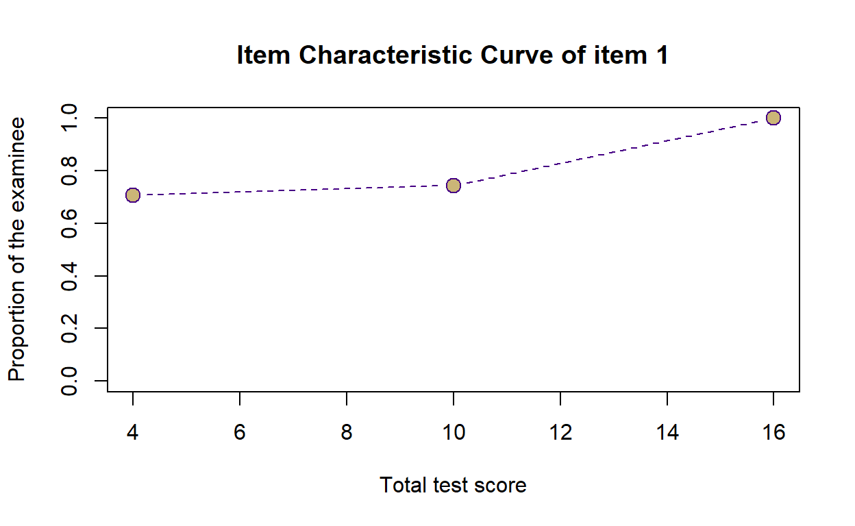
We can also visualize Item Characteristic Curve (ICC) of each item from the scoring output. The x-axis indicates total test score of examinees while the y-axis indicates the proportion of examinee that gets that item right. For example, there are 70% (or 0.7) of examinees who have 4 as their total score got item 1 correctly. The curve goes up as total score of the examinee increases, with the proportion of examinee that gets the item correctly at 100% in examinees with the total score of 16 and above.

Show code

cttICC(score = myScore$score, itemVector = myScore$scored[,1], 
       xlab = "Total test score",
       ylab = "Proportion of the examinee",
       plotTitle = "Item Characteristic Curve of item 1",
       colTheme="dukes", cex=1.5)

We will convert our score data into matrix for for further implementation with item analysis.

Show code

#extract responses only as a matrix
responses <- as.matrix(myScore$scored)

Reliability Analysis

Reliability of a test is an extent to which a test can produce consistent scores for a particular sample of examinees; that is, a test should yield similar, if not the same, scores for an examinee when taken multiple times, given that there is minimal interference such as practice effect. Test reliability can be measured in different ways such as test-retest, internal consistency, or alternate forms.

Internal Consistency

For starter, we will compute internal consistency of the test, which includes Coefficient Alpha (or Cronbach’s Alpha), Guttman’s Lambda-6, Kuder-Richardson 20, and Kuder-Richardson 21. The output also yields the proportion of students who got the item correctly to students who got the item incorrectly as well.

Show code

psych::alpha(myScore$scored, check.keys = T)


Reliability analysis   
Call: psych::alpha(x = myScore$scored, check.keys = T)

  raw_alpha std.alpha G6(smc) average_r S/N   ase mean   sd median_r
      0.55      0.55    0.58     0.057 1.2 0.041 0.48 0.15    0.045

 lower alpha upper     95% confidence boundaries
0.47 0.55 0.63 

 Reliability if an item is dropped:
     raw_alpha std.alpha G6(smc) average_r  S/N alpha se  var.r med.r
V1        0.55      0.54    0.58     0.059 1.18    0.042 0.0081 0.045
V2        0.56      0.55    0.58     0.060 1.21    0.041 0.0079 0.048
V3        0.56      0.55    0.59     0.060 1.22    0.041 0.0080 0.048
V4        0.56      0.56    0.59     0.062 1.25    0.040 0.0080 0.052
V5        0.55      0.54    0.58     0.059 1.20    0.041 0.0081 0.048
V6        0.51      0.50    0.54     0.050 1.00    0.046 0.0071 0.041
V7        0.56      0.55    0.59     0.062 1.25    0.040 0.0078 0.051
V8        0.55      0.54    0.58     0.059 1.19    0.041 0.0080 0.048
V9        0.55      0.54    0.58     0.058 1.17    0.042 0.0080 0.048
V10-      0.56      0.56    0.59     0.062 1.25    0.040 0.0079 0.052
V11       0.54      0.54    0.57     0.057 1.15    0.042 0.0081 0.045
V12       0.55      0.54    0.58     0.058 1.17    0.042 0.0080 0.044
V13       0.53      0.52    0.56     0.055 1.10    0.043 0.0074 0.044
V14       0.53      0.52    0.56     0.055 1.10    0.043 0.0076 0.043
V15       0.54      0.53    0.57     0.057 1.14    0.042 0.0076 0.044
V16       0.51      0.51    0.55     0.051 1.03    0.045 0.0068 0.044
V17       0.49      0.48    0.52     0.047 0.93    0.048 0.0056 0.039
V18       0.51      0.50    0.53     0.050 1.00    0.046 0.0060 0.044
V19       0.55      0.54    0.58     0.059 1.19    0.042 0.0079 0.045
V20       0.55      0.55    0.58     0.060 1.20    0.041 0.0077 0.048

 Item statistics 
       n raw.r std.r r.cor r.drop mean   sd
V1   241  0.26  0.28 0.181  0.125 0.76 0.43
V2   241  0.23  0.24 0.127  0.083 0.73 0.44
V3   241  0.22  0.23 0.115  0.082 0.26 0.44
V4   241  0.20  0.20 0.066  0.043 0.68 0.47
V5   241  0.26  0.26 0.152  0.106 0.37 0.48
V6   241  0.51  0.50 0.497  0.370 0.54 0.50
V7   241  0.19  0.20 0.074  0.045 0.28 0.45
V8   241  0.27  0.27 0.163  0.113 0.48 0.50
V9   241  0.26  0.29 0.199  0.143 0.83 0.38
V10- 241  0.21  0.20 0.067  0.043 0.56 0.50
V11  241  0.32  0.32 0.228  0.169 0.34 0.47
V12  241  0.31  0.30 0.205  0.148 0.56 0.50
V13  241  0.39  0.38 0.323  0.240 0.39 0.49
V14  241  0.40  0.38 0.327  0.247 0.45 0.50
V15  241  0.33  0.33 0.254  0.183 0.31 0.46
V16  241  0.47  0.47 0.452  0.337 0.64 0.48
V17  241  0.60  0.59 0.647  0.478 0.44 0.50
V18  241  0.52  0.50 0.526  0.387 0.33 0.47
V19  241  0.25  0.27 0.176  0.123 0.19 0.39
V20  241  0.26  0.25 0.152  0.097 0.44 0.50

Non missing response frequency for each item
         0    1 miss
 [1,] 0.24 0.76    0
 [2,] 0.27 0.73    0
 [3,] 0.74 0.26    0
 [4,] 0.32 0.68    0
 [5,] 0.63 0.37    0
 [6,] 0.46 0.54    0
 [7,] 0.72 0.28    0
 [8,] 0.52 0.48    0
 [9,] 0.17 0.83    0
[10,] 0.56 0.44    0
[11,] 0.66 0.34    0
[12,] 0.44 0.56    0
[13,] 0.61 0.39    0
[14,] 0.55 0.45    0
[15,] 0.69 0.31    0
[16,] 0.36 0.64    0
[17,] 0.56 0.44    0
[18,] 0.67 0.33    0
[19,] 0.81 0.19    0
[20,] 0.56 0.44    0

Kuder-Richardson

For Kuder-Richardson formula 20 (KR20) and Kuder-Richardson formula 21 (KR21), we can write functions that compute them as follows:

Show code

KR20 <-
  function(X)
    {
    X <- data.matrix(X)
    k <- ncol(X)
    
    # Person total score variances
    SX <- var(rowSums(X))
    
    # item means
    IM <- colMeans(X)
    
    return(((k/(k - 1))*((SX - sum(IM*(1 - IM)))/SX)))
  }

KR20(responses)

[1] 0.541653

Show code

KR21 <-
  function(X)
    {
    X <- data.matrix(X)
    n <- ncol(X)
    
    return((n/(n-1))*((var(rowSums(X)) - n*(sum(colMeans(X))/n) * 
                         (1-(sum(colMeans(X))/n))))/var(rowSums(X)))
  }

KR21(responses)

[1] 0.4700428

Split-half (Test-Retest) Reliability

The test-retest reliability is an estimation of reliability based on the correlation of two equivalent forms of the tests. It is not recommended to use the same test form twice to avoid practice effect, which could artifically increase reliability coefficient of the test.

Show code

psych::splitHalf(scored_item, raw = TRUE, check.keys = TRUE)

Split half reliabilities  
Call: psych::splitHalf(r = scored_item, raw = TRUE, check.keys = TRUE)

Maximum split half reliability (lambda 4) =  0.69
Guttman lambda 6                          =  0.58
Average split half reliability            =  0.55
Guttman lambda 3 (alpha)                  =  0.55
Guttman lambda 2                          =  0.57
Minimum split half reliability  (beta)    =  0.31
Average interitem r =  0.06  with median =  0.04
                                             2.5% 50% 97.5%
 Quantiles of split half reliability      =  0.44 0.55 0.63

Spearman-Brown Reliability

To compute Spearman-Brown reliability, we need to use Cronbach’s Alpha as a base computation; for that, we need to export the function as a separate file first.

Show code

#With a written function
cronbachs.alpha <-
  function(X)
    {
    
    X <- data.matrix(X)
    n <- ncol(X) # Number of items
    k <- nrow(X) # Number of examinees
    
    # Cronbachs alpha
    alpha <- (n/(n - 1))*(1 - sum(apply(X, 2, var))/var(rowSums(X)))
    
    return(list("Crombach's alpha" = alpha,
                "Number of items" = n,
                "Number of examinees" = k))
    }

#Dump "cronbach.alpha" function for further use
dump("cronbachs.alpha", file = "cronbachs.alpha.R")

The Spearman-Brown prophecy formula is a formula that predicts reliability of the test through the modification of test length. This formula is one way can use to answer questions such as “how short can I make my assessment?” or “how many items should I write for my test to have adequate reliability?”
Reliability of a test usually decreases when we shorten the test length and increases when we add more test items as well. However, there is no magic number of how long a test should be, so one should consider their context such as nature of the test content, ability of the examinee, and average time for a student to complete the assessment.

Show code

SpearmanBrown <- 
  function(x, n1, n2)
    {
    
    source("cronbachs.alpha.R")
    
    x <- as.matrix(x)
    N <- n2/n1
    
    # cronbach's alpha for the original test
    alpha <- cronbachs.alpha(x)[[1]]
    predicted.alpha <- N * alpha / (1 + (N - 1) * alpha)
    
    return(list(original.reliability = alpha,
                original.sample.size = n1,
                predicted.reliability = predicted.alpha,
                predicted.sample.size = n2))
  }

# predict reliability by Spearman-Brown formula
# if the number of items is reduced from 25 to 15
SpearmanBrown(responses, n1 = 20, n2 = 15)

$original.reliability
[1] 0.5395239

$original.sample.size
[1] 20

$predicted.reliability
[1] 0.4677309

$predicted.sample.size
[1] 15

Show code

# predict reliability by Spearman-Brown formula
# if the number of items is increased from 25 to 35
SpearmanBrown(responses, n1 = 20, n2 = 35)

$original.reliability
[1] 0.5395239

$original.sample.size
[1] 20

$predicted.reliability
[1] 0.6721757

$predicted.sample.size
[1] 35

Show code

# predict reliability by Spearman-Brown formula
# if the number of items is doubled
SpearmanBrown(responses, n1 = 20, n2 = 40)

$original.reliability
[1] 0.5395239

$original.sample.size
[1] 20

$predicted.reliability
[1] 0.7008971

$predicted.sample.size
[1] 40

Guttman’s Lambda

Guttman’s Lambda is also another reliability coefficient we can use in similar way as Coefficient Alpha (or Cronbach’s Alpha).

Show code

psych::guttman(responses)

Call: psych::guttman(r = responses)

Alternative estimates of reliability

Guttman bounds 
L1 =  0.51 
L2 =  0.56 
L3 (alpha) =  0.53 
L4 (max) =  0.69 
L5 =  0.55 
L6 (smc) =  0.57 
TenBerge bounds 
mu0 =  0.53 mu1 =  0.56 mu2 =  0.56 mu3 =  0.56 

alpha of first PC =  0.64 
estimated greatest lower bound based upon communalities=  0.69 

beta found by splitHalf  =  0.32

Pearson product-moment correlation coefficient

Another way we can compute reliability of the test is via Pearson product-moment correlation between two halves of the test (aka Split-half method). However, comparing only a pair or two of the test half might not be enough. We can use Bootstrap resampling method to randomly split the examinees into two halves 1000 times, so that we can make sure that the computation is as exhaustive as possible.

Show code

#Split data (variables-item) into two equally and randomly.

split.items <- 
  function(X, seed = NULL)
    {
    # optional fixed seed
    if (!is.null(seed)) {set.seed(seed)} 
    
    X <- as.matrix(X)
    
    # if n = 2x, then lengths Y1 = Y2
    # if n = 2x+1, then lenths Y1 = Y2+1
    n <- ncol(X)
    index <- sample(1:n, ceiling(n/2))
    Y1 <- X[, index ]
    Y2 <- X[, -index]
    return(list(Y1, Y2)) 
  }

dump("split.items", file = "split.items.R")

Show code

pearson <- 
  function(X, seed = NULL, n = NULL)
    {
    source("split.items.R")
    
    # optional fixed seed
    if (!is.null(seed)) {set.seed(seed)}
    
    # the number of bootstrap replicates. 1e3 = 1000
    if (is.null(n)) {n <- 1e3}   
    
    X <- as.matrix(X)
    r <- rep(NA, n)
    
    for (i in 1:n) {
      # split items
      Y <- split.items(X)
      
      # total scores
      S1 <- as.matrix(rowSums(Y[[1]]))
      S2 <- as.matrix(rowSums(Y[[2]]))
      
      # residual scores
      R1 <- S1 - mean(S1)
      R2 <- S2 - mean(S2)
      
      # Pearson product-moment correlation coefficient
      r[i] <- (t(R1) %*% R2) / (sqrt((t(R1) %*% R1)) * sqrt((t(R2) %*% R2)))
    }
    
    return(mean(r))
  }

# compute the Pearson product-moment correlation coefficient
pearson(responses, seed = 456, n = 1)

[1] 0.3499066

We can also double check if the function is right by splitting response of the examinee into two halves and compute a correlation coefficient by ourselves.

Show code

# compare
# split items
set.seed(456)
Y <- split.items(responses)

# total scores
Set1 <- as.matrix(rowSums(Y[[1]]))
Set2 <- as.matrix(rowSums(Y[[2]]))

cor(Set1, Set2)

          [,1]
[1,] 0.3499066

Note that the split-half method can both overestimate or underestimate ability of the examinees when two halves of the test are not parallel.

Standard Error of Measurement

Standard error of measurement is a measure of the spread of observed score around the “true” score. The standard error of measurement that uses Coefficient’s alpha as its reliability statistics can be computed as follows:

Show code

SEM <-
  function(X){
    source("cronbachs.alpha.R")
    X <- data.matrix(X)
    
    return(sd(rowSums(X)) * sqrt(1 - cronbachs.alpha(X)[[1]]))
  }

SEM(responses)

[1] 2.036401

As a result, the range in which the true score of an examinee might stay in could be ± 2.036401.

Confidence Intervals for True Scores

We can also compute confidence interval for true scores of each item via the code below. Note that one limitation of CTT is that it is population dependent, so the confidence interval may change when the test is administered to a different group of examinees.

Show code

# 90% confidence interval for the true score
head(cbind(lower_bound = round(rowSums(responses)-1.65* sd(rowSums(responses))*
                                 sqrt(1-KR20(responses)), 2), observed = rowSums(responses),
           upper_bound = round(rowSums(responses)+1.65* sd(rowSums(responses))*
                                 sqrt(1-KR20(responses)), 2)), 20)

      lower_bound observed upper_bound
 [1,]        5.65        9       12.35
 [2,]        2.65        6        9.35
 [3,]        9.65       13       16.35
 [4,]        5.65        9       12.35
 [5,]       10.65       14       17.35
 [6,]        8.65       12       15.35
 [7,]        3.65        7       10.35
 [8,]        5.65        9       12.35
 [9,]        4.65        8       11.35
[10,]        7.65       11       14.35
[11,]        2.65        6        9.35
[12,]        4.65        8       11.35
[13,]        1.65        5        8.35
[14,]        9.65       13       16.35
[15,]        4.65        8       11.35
[16,]        1.65        5        8.35
[17,]       11.65       15       18.35
[18,]        4.65        8       11.35
[19,]        6.65       10       13.35
[20,]        9.65       13       16.35

Item Analysis

- Item Analysis of the Classical Test Theory approach relies on two statistics to evaluate an item, P-value (not to be confused with p-value in statistical tests) and point-biserial correlation coefficient (p-Bis).
P-value in this context represents the proportion of examinees responding in the keyed direction It is typically referred to as item difficulty. Point-biserial corrrelation coefficient is the correlation between a particular item and other items; this index is typically referred to as item discrimination that indicates the degree to which that item can distinguish high ability examinee or examinees who actually know that construct from examinees who do not possess adequate knowledge to get that item correctly.

Item Discrimination.

As mentioned above, item discrimination refers to how well an item discriminates high-ability examinees from those with low-ability. Items that are very hard (i.e., p < 0.20) or very easy (p > 0.90) usually have lower item discrimination values than items with medium difficulty.
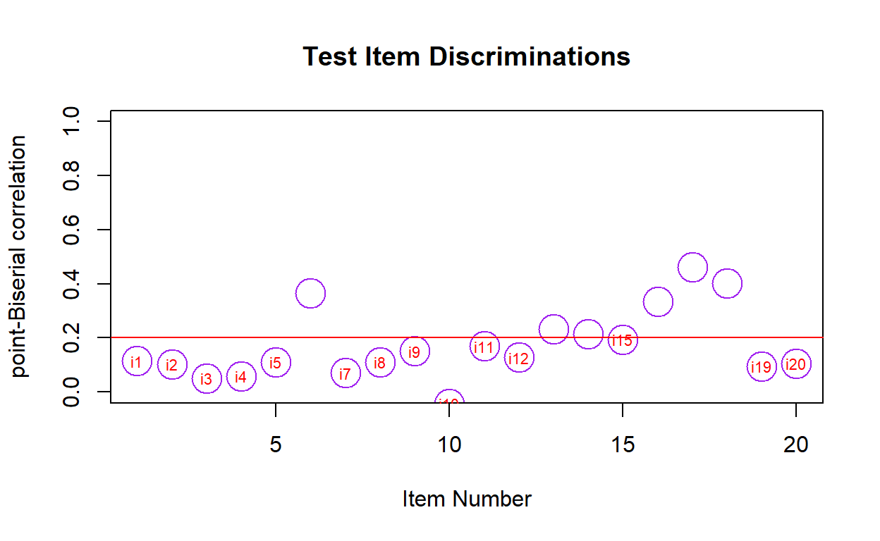
We usually examine point-biserial correlation coefficient (p-Bis) of the item. If p-Bis is lower than 0.20, the item can be flagged for low discrimination, while 0.20 to 0.39 indicates good discrimination, and 0.4 and above indicates excellent discrimination. If p-Bis is negative, then the item doesn’t seem to measure the same construct that the other items are measuring. It could also mean that the item is mis-keyed.

Show code

item.analysis <- 
  function(responses)
    {
    # CRITICAL VALUES
    cvpb = 0.20
    cvdl = 0.15
    cvdu = 0.85
    
    require(CTT, warn.conflicts = FALSE, quietly = TRUE)
    (ctt.analysis <- CTT::reliability(responses, itemal = TRUE, NA.Delete = TRUE))
    
    # Mark items that are potentially problematic
    item.analysis <- data.frame(item = seq(1:ctt.analysis$nItem),
                                r.pbis = ctt.analysis$pBis,
                                bis = ctt.analysis$bis,
                                item.mean = ctt.analysis$itemMean,
                                alpha.del = ctt.analysis$alphaIfDeleted)
  
    if (TRUE) {
      item.analysis$check <- 
        ifelse(item.analysis$r.pbis < cvpb |
                 item.analysis$item.mean < cvdl |
                 item.analysis$item.mean > cvdu, "X", "")
    }
    
    return(item.analysis)
  }

kbl(item.analysis(responses)) %>%
  kable_styling(bootstrap_options = c("striped", "hover", "condensed", "responsive"),
                full_width = FALSE, position = "left")

item	r.pbis	bis	item.mean	alpha.del	check
1	0.1147596	0.1683232	0.7593361	0.5353385	X
2	0.1035530	0.1409292	0.7344398	0.5372914	X
3	0.0506175	0.0685887	0.2572614	0.5452346	X
4	0.0591143	0.0785356	0.6804979	0.5450389	X
5	0.1111202	0.1406669	0.3651452	0.5369402	X
6	0.3656502	0.4640379	0.5394191	0.4909063
7	0.0700444	0.0920897	0.2780083	0.5426513	X
8	0.1112357	0.1394688	0.4813278	0.5373705	X
9	0.1515853	0.2230714	0.8298755	0.5299043	X
10	-0.0434185	-0.0549382	0.4356846	0.5634988	X
11	0.1696824	0.2157830	0.3360996	0.5269375	X
12	0.1279600	0.1627060	0.5601660	0.5343645	X
13	0.2312726	0.2933878	0.3900415	0.5161192
14	0.2134979	0.2656683	0.4481328	0.5191567
15	0.1947141	0.2547864	0.3112033	0.5227779	X
16	0.3353941	0.4428850	0.6390041	0.4977310
17	0.4609036	0.5799529	0.4356846	0.4727918
18	0.4013261	0.5080745	0.3319502	0.4865119
19	0.0956187	0.1323704	0.1908714	0.5375545	X
20	0.1054536	0.1323520	0.4356846	0.5382775	X

Item Difficulty

Under CTT, item difficulty is simply the percentages of examinees obtaining the correct answer. Item difficulty ranges from 0 to 1, with higher values indicate easier items as more examinees are able to correctly answer this item. This index is useful in assessing whether it is appropriate for the level of the students taking the test.
The desired range of item difficulty index is between 0.3 to 0.9 (by approximate), while the number close to 0 or 1 offers little information on measuring students’ level of the construct. In plain words, we wouldn’t want to have test items that are too easy that everybody get it right, or items that are too hard that no one can answer it correctly. However, the extreme cut-off for item difficulty could apply to measurements that are designed for extreme groups.

Show code

Item_Difficulty <- item.exam(x = responses, y = NULL, discrim = T)

kbl(Item_Difficulty) %>%
  kable_styling(bootstrap_options = c("striped", "hover", "condensed", "responsive"),
                full_width = FALSE, position = "left")

Sample.SD	Item.total	Item.Tot.woi	Difficulty	Discrimination	Item.Criterion	Item.Reliab	Item.Rel.woi	Item.Validity
0.4283763	0.2544665	0.1147596	0.7593361	0.2125	NA	0.1087810	0.0490582	NA
0.4425501	0.2483214	0.1035530	0.7344398	0.2875	NA	0.1096664	0.0457322	NA
0.4380344	0.1956677	0.0506175	0.2572614	0.2375	NA	0.0855312	0.0221262	NA
0.4672541	0.2135535	0.0591143	0.6804979	0.2125	NA	0.0995765	0.0275640	NA
0.4824729	0.2684805	0.1111202	0.3651452	0.3125	NA	0.1292655	0.0535011	NA
0.4994811	0.5054235	0.3656502	0.5394191	0.5500	NA	0.2519252	0.1822561	NA
0.4489499	0.2181283	0.0700444	0.2780083	0.1625	NA	0.0977253	0.0313811	NA
0.5006911	0.2744754	0.1112357	0.4813278	0.3125	NA	0.1371420	0.0555790	NA
0.3765241	0.2730001	0.1515853	0.8298755	0.2375	NA	0.1025776	0.0569570	NA
0.4968782	0.1224407	-0.0434185	0.4356846	0.1375	NA	0.0607118	-0.0215289	NA
0.4733565	0.3208135	0.1696824	0.3360996	0.3125	NA	0.1515438	0.0801535	NA
0.4973999	0.2892525	0.1279600	0.5601660	0.2625	NA	0.1435753	0.0635151	NA
0.4887744	0.3825120	0.2312726	0.3900415	0.4000	NA	0.1865738	0.1128054	NA
0.4983375	0.3691600	0.2134979	0.4481328	0.4750	NA	0.1835842	0.1061730	NA
0.4639493	0.3412014	0.1947141	0.3112033	0.3625	NA	0.1579714	0.0901499	NA
0.4812889	0.4738815	0.3353941	0.6390041	0.4750	NA	0.2276002	0.1610862	NA
0.4968782	0.5863010	0.4609036	0.4356846	0.6125	NA	0.2907152	0.2285373	NA
0.4718933	0.5290626	0.4013261	0.3319502	0.5000	NA	0.2491426	0.1889898	NA
0.3938058	0.2248264	0.0956187	0.1908714	0.1500	NA	0.0883541	0.0375770	NA
0.4968782	0.2677464	0.1054536	0.4356846	0.3125	NA	0.1327610	0.0522888	NA

Visualizing Item Discrimination

We can use the functions below to visualize for items that should be revised for low discrimination power

Show code

item.discrimination <-
  function(responses)
    {
    # CRITICAL VALUES
    cvpb = 0.20
    cvdl = 0.15
    cvdu = 0.85
    
    require(CTT, warn.conflicts = FALSE, quietly = TRUE)
    ctt.analysis <- CTT::reliability(responses, itemal = TRUE, NA.Delete = TRUE)
    
    item.discrimination <- data.frame(item = 1:ctt.analysis$nItem , 
                                      discrimination = ctt.analysis$pBis)
    
    plot(item.discrimination,
         type = "p",
         pch = 1,
         cex = 3,
         col = "purple",
         ylab = "point-Biserial correlation",
         xlab = "Item Number",
         ylim = c(0, 1),
         main = "Test Item Discriminations")
    
    abline(h = cvpb, col = "red")
    
    outlier <- data.matrix(subset(item.discrimination,
                                  subset = (item.discrimination[, 2] < cvpb)))
    
    text(outlier, paste("i", outlier[,1], sep = ""), col = "red", cex = .7)
    
    return(item.discrimination[order(item.discrimination$discrimination),])
  }

item.discrimination(responses)

   item discrimination
10   10    -0.04341855
3     3     0.05061749
4     4     0.05911432
7     7     0.07004435
19   19     0.09561872
2     2     0.10355300
20   20     0.10545357
5     5     0.11112015
8     8     0.11123568
1     1     0.11475958
12   12     0.12795997
9     9     0.15158531
11   11     0.16968243
15   15     0.19471413
14   14     0.21349786
13   13     0.23127262
16   16     0.33539410
6     6     0.36565023
18   18     0.40132606
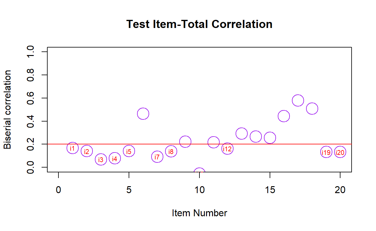
17   17     0.46090362

Visualizing Item Total-Correlation (Bis)

The item total correlation is a correlation between the question score (e.g., 0 or 1 for multiple choice) and the overall assessment score. The assumption is that if an examinee gets a question correctly they should, in general, have higher overall assessment scores than participants who get that question wrong.

Show code

test_item.total <-
  function(responses)
    {
    # CRITICAL VALUES
    cvpb = 0.20
    cvdl = 0.15
    cvdu = 0.85
    
    require(CTT, warn.conflicts = FALSE, quietly = TRUE)
    ctt.analysis <- CTT::reliability(responses, itemal = TRUE, NA.Delete = TRUE)
    
    test_item.total <- data.frame(item = 1:ctt.analysis$nItem , 
                                  biserial = ctt.analysis$bis)
    
    plot(test_item.total,
         main = "Test Item-Total Correlation",
         type = "p",
         pch = 1,
         cex = 2.8,
         col = "purple",
         ylab = "Biserial correlation",
         xlab = "Item Number",
         ylim = c(0, 1),
         xlim = c(0, ctt.analysis$nItem))
    
    abline(h = cvpb, col = "red")
    
    outlier <- data.matrix(subset(test_item.total,
                                  subset = test_item.total[,2] < cvpb))
    
    text(outlier, paste("i", outlier[,1], sep = ""), col = "red", cex = .7)
    
    return(test_item.total[order(test_item.total$biserial),])
    }

test_item.total(responses)

   item    biserial
10   10 -0.05493825
3     3  0.06858871
4     4  0.07853557
7     7  0.09208970
20   20  0.13235198
19   19  0.13237037
8     8  0.13946879
5     5  0.14066694
2     2  0.14092920
12   12  0.16270597
1     1  0.16832321
11   11  0.21578295
9     9  0.22307140
15   15  0.25478638
14   14  0.26566826
13   13  0.29338781
16   16  0.44288497
6     6  0.46403793
18   18  0.50807452
17   17  0.57995293

Distractor/Option Analysis

In distractor analysis, examinees are divided into three ability levels (i.e., lower, middle and upper) based on their total test score. The proportions of examinees who mark each option in each of the three ability levels are compared. In the lower ability level, we would expect to see a smaller proportion of examinees choosing the correct option and a larger proportion of them choosing the incorrect options (known as distractors).
Ideally, good distractors would attract about the same proportion of examinees. Distractors that don’t attract any or attract a very small proportion of examinees relative to other distractors should be considered for revision. We do not want response options that are too obvious.
In those with higher ability level, we would expect to see the majority of examinees choose the correct option. If distractors are more appealing than the correct option to high ability examineess, then it should be eliminated or revised.

Show code

distractorAnalysis(items = data, key = key, nGroups = 4, pTable = T)

$i001
  correct key   n       rspP       pBis     discrim      lower
A       *   A 183 0.75933610  0.1147596  0.22334218 0.70769231
B           B  16 0.06639004 -0.2888067 -0.13846154 0.13846154
C           C  22 0.09128631 -0.1975788 -0.05968170 0.07692308
D           D  20 0.08298755 -0.1841578 -0.02519894 0.07692308
       mid50      mid75      upper
A 0.63636364 0.78846154 0.93103448
B 0.06060606 0.05769231 0.00000000
C 0.16666667 0.09615385 0.01724138
D 0.13636364 0.05769231 0.05172414

$i002
  correct key   n       rspP        pBis     discrim      lower
A           A   8 0.03319502 -0.01743924  0.01909814 0.01538462
B           B  40 0.16597510 -0.28940212 -0.16180371 0.23076923
C       *   C 177 0.73443983  0.10355300  0.26392573 0.61538462
D           D  16 0.06639004 -0.28880672 -0.12122016 0.13846154
       mid50      mid75      upper
A 0.01515152 0.07692308 0.03448276
B 0.16666667 0.19230769 0.06896552
C 0.74242424 0.71153846 0.87931034
D 0.07575758 0.01923077 0.01724138

$i003
  correct key  n      rspP        pBis     discrim     lower
A           A 61 0.2531120 -0.21045253 -0.05278515 0.2769231
B           B 74 0.3070539 -0.32875754 -0.22387268 0.4307692
C       *   C 62 0.2572614  0.05061749  0.16021220 0.1846154
D           D 44 0.1825726 -0.04787523  0.11644562 0.1076923
      mid50     mid75     upper
A 0.2878788 0.2115385 0.2241379
B 0.2878788 0.2884615 0.2068966
C 0.1818182 0.3461538 0.3448276
D 0.2424242 0.1538462 0.2241379

$i004
  correct key   n       rspP        pBis     discrim      lower
A           A  11 0.04564315 -0.16015191 -0.09045093 0.10769231
B           B  24 0.09958506 -0.15640748 -0.04244032 0.07692308
C           C  42 0.17427386 -0.28460760 -0.15437666 0.29230769
D       *   D 164 0.68049793  0.05911432  0.28726790 0.52307692
      mid50      mid75      upper
A 0.0000000 0.05769231 0.01724138
B 0.1515152 0.13461538 0.03448276
C 0.1363636 0.11538462 0.13793103
D 0.7121212 0.69230769 0.81034483

$i005
  correct key  n       rspP       pBis     discrim      lower
A           A 84 0.34854772 -0.2097597 -0.02997347 0.32307692
B       *   B 88 0.36514523  0.1111202  0.27294430 0.26153846
C           C 61 0.25311203 -0.3237027 -0.19681698 0.36923077
D           D  8 0.03319502 -0.1706663 -0.04615385 0.04615385
       mid50      mid75     upper
A 0.42424242 0.34615385 0.2931034
B 0.22727273 0.48076923 0.5344828
C 0.30303030 0.13461538 0.1724138
D 0.04545455 0.03846154 0.0000000

$i006
  correct key   n       rspP       pBis    discrim     lower
A           A  61 0.25311203 -0.3587149 -0.2503979 0.3538462
B       *   B 130 0.53941909  0.3656502  0.6466844 0.2153846
C           C  34 0.14107884 -0.3800902 -0.2615385 0.2615385
D           D  16 0.06639004 -0.2994444 -0.1347480 0.1692308
       mid50      mid75      upper
A 0.34848485 0.17307692 0.10344828
B 0.45454545 0.69230769 0.86206897
C 0.16666667 0.11538462 0.00000000
D 0.03030303 0.01923077 0.03448276

$i007
  correct key  n      rspP        pBis      discrim     lower
A       *   A 67 0.2780083  0.07004435  0.211936340 0.1846154
B           B 63 0.2614108 -0.17772394  0.027851459 0.2307692
C           C 47 0.1950207 -0.13004489  0.003183024 0.1692308
D           D 64 0.2655602 -0.32387947 -0.242970822 0.4153846
      mid50     mid75     upper
A 0.2424242 0.3076923 0.3965517
B 0.3333333 0.2115385 0.2586207
C 0.1818182 0.2692308 0.1724138
D 0.2424242 0.2115385 0.1724138

$i008
  correct key   n       rspP        pBis     discrim      lower
A           A  61 0.25311203 -0.45040855 -0.34641910 0.41538462
B           B  53 0.21991701 -0.11191555  0.01061008 0.23076923
C       *   C 116 0.48132780  0.11123568  0.36286472 0.29230769
D           D  11 0.04564315 -0.08820493 -0.02705570 0.06153846
       mid50      mid75      upper
A 0.34848485 0.13461538 0.06896552
B 0.16666667 0.25000000 0.24137931
C 0.42424242 0.59615385 0.65517241
D 0.06060606 0.01923077 0.03448276

$i009
  correct key   n       rspP       pBis     discrim      lower
A           A   8 0.03319502 -0.1554692 -0.04244032 0.07692308
B       *   B 200 0.82987552  0.1515853  0.28488064 0.64615385
C           C  19 0.07883817 -0.2169620 -0.15013263 0.18461538
D           D  14 0.05809129 -0.2866682 -0.09230769 0.09230769
       mid50      mid75      upper
A 0.01515152 0.00000000 0.03448276
B 0.87878788 0.88461538 0.93103448
C 0.01515152 0.07692308 0.03448276
D 0.09090909 0.03846154 0.00000000

$i010
  correct key   n       rspP        pBis     discrim     lower
A           A  94 0.39004149 -0.13702229  0.02360743 0.3384615
B           B  23 0.09543568 -0.16743006 -0.05596817 0.1076923
C           C  19 0.07883817 -0.27622610 -0.13474801 0.1692308
D       *   D 105 0.43568465 -0.04341855  0.16710875 0.3846154
       mid50      mid75      upper
A 0.43939394 0.42307692 0.36206897
B 0.07575758 0.15384615 0.05172414
C 0.04545455 0.05769231 0.03448276
D 0.43939394 0.36538462 0.55172414

$i011
  correct key   n       rspP       pBis     discrim     lower
A           A 117 0.48547718 -0.3887571 -0.29151194 0.5846154
B           B  23 0.09543568 -0.1398436 -0.02148541 0.1076923
C       *   C  81 0.33609959  0.1696824  0.38435013 0.1846154
D           D  20 0.08298755 -0.1548240 -0.07135279 0.1230769
       mid50      mid75      upper
A 0.59090909 0.44230769 0.29310345
B 0.12121212 0.05769231 0.08620690
C 0.21212121 0.42307692 0.56896552
D 0.07575758 0.07692308 0.05172414

$i012
  correct key   n       rspP       pBis     discrim     lower
A       *   A 135 0.56016598  0.1279600  0.32413793 0.4000000
B           B  59 0.24481328 -0.2253473 -0.03925729 0.2461538
C           C  24 0.09958506 -0.2766477 -0.16737401 0.1846154
D           D  23 0.09543568 -0.2673278 -0.11750663 0.1692308
       mid50      mid75      upper
A 0.50000000 0.65384615 0.72413793
B 0.31818182 0.19230769 0.20689655
C 0.09090909 0.09615385 0.01724138
D 0.09090909 0.05769231 0.05172414

$i013
  correct key  n      rspP       pBis    discrim     lower     mid50
A           A 27 0.1120332 -0.2781623 -0.1501326 0.1846154 0.1363636
B           B 46 0.1908714 -0.1753162 -0.1100796 0.2307692 0.1212121
C           C 74 0.3070539 -0.3778479 -0.2564987 0.4461538 0.3333333
D       *   D 94 0.3900415  0.2312726  0.5167109 0.1384615 0.4090909
       mid75      upper
A 0.07692308 0.03448276
B 0.30769231 0.12068966
C 0.23076923 0.18965517
D 0.38461538 0.65517241

$i014
  correct key   n      rspP       pBis    discrim     lower     mid50
A       *   A 108 0.4481328  0.2134979  0.5358090 0.1538462 0.4393939
B           B  31 0.1286307 -0.2535706 -0.1445623 0.2307692 0.1060606
C           C  58 0.2406639 -0.3415163 -0.2774536 0.4153846 0.2121212
D           D  44 0.1825726 -0.2361190 -0.1137931 0.2000000 0.2424242
       mid75     upper
A 0.55769231 0.6896552
B 0.07692308 0.0862069
C 0.17307692 0.1379310
D 0.19230769 0.0862069

$i015
  correct key  n       rspP       pBis     discrim      lower
A           A 15 0.06224066 -0.1403108 -0.02148541 0.10769231
B           B 74 0.30705394 -0.3315040 -0.24111406 0.43076923
C       *   C 75 0.31120332  0.1947141  0.40769231 0.09230769
D           D 77 0.31950207 -0.2661525 -0.14509284 0.36923077
       mid50      mid75     upper
A 0.03030303 0.01923077 0.0862069
B 0.31818182 0.26923077 0.1896552
C 0.30303030 0.38461538 0.5000000
D 0.34848485 0.32692308 0.2241379

$i016
  correct key   n       rspP       pBis     discrim      lower
A       *   A 154 0.63900415  0.3353941  0.59071618 0.32307692
B           B  39 0.16182573 -0.4136149 -0.31750663 0.36923077
C           C  11 0.04564315 -0.1861371 -0.06153846 0.06153846
D           D  37 0.15352697 -0.3545356 -0.21167109 0.24615385
       mid50      mid75      upper
A 0.56060606 0.82692308 0.91379310
B 0.13636364 0.05769231 0.05172414
C 0.09090909 0.01923077 0.00000000
D 0.21212121 0.09615385 0.03448276

$i017
  correct key   n      rspP       pBis    discrim     lower
A           A  82 0.3402490 -0.4829386 -0.4350133 0.5384615
B           B  26 0.1078838 -0.3113845 -0.1538462 0.1538462
C       *   C 105 0.4356846  0.4609036  0.7716180 0.1076923
D           D  28 0.1161826 -0.2706021 -0.1827586 0.2000000
       mid50      mid75      upper
A 0.36363636 0.32692308 0.10344828
B 0.21212121 0.03846154 0.00000000
C 0.33333333 0.48076923 0.87931034
D 0.09090909 0.15384615 0.01724138

$i018
  correct key  n       rspP       pBis    discrim      lower
A           A 96 0.39834025 -0.4250997 -0.3180371 0.50769231
B           B 43 0.17842324 -0.2755281 -0.1925729 0.26153846
C           C 22 0.09128631 -0.2623175 -0.1366048 0.15384615
D       *   D 80 0.33195021  0.4013261  0.6472149 0.07692308
       mid50      mid75      upper
A 0.48484848 0.38461538 0.18965517
B 0.18181818 0.19230769 0.06896552
C 0.09090909 0.09615385 0.01724138
D 0.24242424 0.32692308 0.72413793

$i019
  correct key   n       rspP        pBis     discrim     lower
A           A  17 0.07053942 -0.14630133 -0.07135279 0.1230769
B           B  48 0.19917012 -0.23586731 -0.09469496 0.2153846
C           C 130 0.53941909 -0.22016521 -0.05570292 0.5384615
D       *   D  46 0.19087137  0.09561872  0.22175066 0.1230769
       mid50      mid75      upper
A 0.06060606 0.03846154 0.05172414
B 0.22727273 0.23076923 0.12068966
C 0.57575758 0.55769231 0.48275862
D 0.13636364 0.17307692 0.34482759

$i020
  correct key   n       rspP       pBis     discrim      lower
A           A  21 0.08713693 -0.2194626 -0.07506631 0.09230769
B           B  49 0.20331950 -0.1948577 -0.07374005 0.24615385
C       *   C 105 0.43568465  0.1054536  0.32838196 0.29230769
D           D  66 0.27385892 -0.2973162 -0.17957560 0.36923077
      mid50      mid75      upper
A 0.1515152 0.07692308 0.01724138
B 0.1969697 0.19230769 0.17241379
C 0.3939394 0.46153846 0.62068966
D 0.2575758 0.26923077 0.18965517

Concluding remark

While we have discussed a lot about characteristics of test items such as Reliability, Item Difficulty, and Item Discrimination, those concepts are building blocks of a bigger concept known as test validity. Test Validity is the foundational concept in measurement that concerns the evidential support to the interpretation and use score of a test score in a particular context (AERA et al., 2014);
For example, in order to use WAIS-IV for diagnostic purposes in Thailand, an array of validity evidence needs to be established such as evidence based on test content (i.e., is content of the test known to the Thai population?), evidence based on internal structure of the test (i.e., how do we know if items of the test measure the same psychological attribute?), or even evidence based on consequences of the test (i.e., are we sure that claims made from the test such as learning disability diagnosis are for that purpose only and for no other unrelated claims such as stigmatization?).
CTT is relatively weak in its theoretical assumption, which makes it applicable to many testing situations. This framework also does not require a complex theoretical model to assess psychological attributes of examinees. However, CTT falls short in its sample dependency, which makes it less preferable in test development scenarios that require associations with other population such as test equating and computerized adaptive testing. Item Response Theory is able to address this limitation.
With online assessment becoming more implemented, especially in this pandemic time where most activities take place in online environments, we can take advantage of the technology by having computers score the exam for us for improved efficiency. We can also improve property of our test by using information from item analysis as demonstrated above as well. While testing brings about anxiety in a lot of students (me included. I hate being tested), we can hardly deny that it is an important part of education and other settings (e.g., clinical, legal). For that, it is important that every decision made on the test needs to be supported by as much evidence as possible. As always, thank you very much for checking this post out. Good day, everyone!

Comment on this article Share:

Classical Test Theory in R

Introduction

Reliability Analysis

Internal Consistency

Kuder-Richardson

Split-half (Test-Retest) Reliability

Spearman-Brown Reliability

Guttman’s Lambda

Pearson product-moment correlation coefficient

Standard Error of Measurement

Confidence Intervals for True Scores

Item Analysis

Item Discrimination.

Item Difficulty

Visualizing Item Discrimination

Visualizing Item Total-Correlation (Bis)

Distractor/Option Analysis

Concluding remark

Reuse

Citation

i001	i002	i003	i004	i005	i006	i007	i008	i009	i010	i011	i012	i013	i014	i015	i016	i017	i018	i019	i020
A	C	D	D	A	B	C	A	B	A	A	B	D	C	B	A	C	D	C	D
B	C	B	D	C	C	A	A	B	D	A	C	D	B	B	B	A	A	C	D
A	C	B	D	B	A	A	C	B	D	C	A	D	A	C	B	A	C	C	B
A	C	B	D	B	A	A	A	B	D	A	D	B	D	C	D	A	A	C	C
A	C	D	D	A	B	B	A	B	A	C	A	D	A	C	A	C	D	C	C
A	C	B	D	C	B	C	C	B	A	C	B	D	A	C	A	C	B	C	D

V1	V2	V4	V5	V6	V7	V8	V9	V10	V11	V12	V13	V14	V15	V16	V17	V18	V20
1	1	1	0	1	0	0	1	0	0	0	1	0	0	1	1	1	0
0	1	1	0	0	1	0	1	1	0	0	1	0	0	0	0	0	0
1	1	1	1	0	1	1	1	1	1	1	1	1	1	0	0	0	0
1	1	1	1	0	1	0	1	1	0	0	0	0	1	0	0	0	1
1	1	1	0	1	0	0	1	0	1	1	1	1	1	1	1	1	1
1	1	1	0	1	0	1	1	0	1	0	1	1	1	1	1	0	0

i001	i002	i003	i004	i005	i006	i007	i008	i009	i010	i011	i012	i013	i014	i015	i016	i017	i018	i019	i020
A	C	D	D	A	B	C	A	B	A	A	B	D	C	B	A	C	D	C	D
B	C	B	D	C	C	A	A	B	D	A	C	D	B	B	B	A	A	C	D
A	C	B	D	B	A	A	C	B	D	C	A	D	A	C	B	A	C	C	B
A	C	B	D	B	A	A	A	B	D	A	D	B	D	C	D	A	A	C	C
A	C	D	D	A	B	B	A	B	A	C	A	D	A	C	A	C	D	C	C
A	C	B	D	C	B	C	C	B	A	C	B	D	A	C	A	C	B	C	D

V1	V2	V4	V5	V6	V7	V8	V9	V10	V11	V12	V13	V14	V15	V16	V17	V18	V20
1	1	1	0	1	0	0	1	0	0	0	1	0	0	1	1	1	0
0	1	1	0	0	1	0	1	1	0	0	1	0	0	0	0	0	0
1	1	1	1	0	1	1	1	1	1	1	1	1	1	0	0	0	0
1	1	1	1	0	1	0	1	1	0	0	0	0	1	0	0	0	1
1	1	1	0	1	0	0	1	0	1	1	1	1	1	1	1	1	1
1	1	1	0	1	0	1	1	0	1	0	1	1	1	1	1	0	0

i001	i002	i003	i004	i005	i006	i007	i008	i009	i010	i011	i012	i013	i014	i015	i016	i017	i018	i019	i020
A	C	D	D	A	B	C	A	B	A	A	B	D	C	B	A	C	D	C	D
B	C	B	D	C	C	A	A	B	D	A	C	D	B	B	B	A	A	C	D
A	C	B	D	B	A	A	C	B	D	C	A	D	A	C	B	A	C	C	B
A	C	B	D	B	A	A	A	B	D	A	D	B	D	C	D	A	A	C	C
A	C	D	D	A	B	B	A	B	A	C	A	D	A	C	A	C	D	C	C
A	C	B	D	C	B	C	C	B	A	C	B	D	A	C	A	C	B	C	D

V1	V2	V4	V5	V6	V7	V8	V9	V10	V11	V12	V13	V14	V15	V16	V17	V18	V20
1	1	1	0	1	0	0	1	0	0	0	1	0	0	1	1	1	0
0	1	1	0	0	1	0	1	1	0	0	1	0	0	0	0	0	0
1	1	1	1	0	1	1	1	1	1	1	1	1	1	0	0	0	0
1	1	1	1	0	1	0	1	1	0	0	0	0	1	0	0	0	1
1	1	1	0	1	0	0	1	0	1	1	1	1	1	1	1	1	1
1	1	1	0	1	0	1	1	0	1	0	1	1	1	1	1	0	0