Examining PISA 2018 Data Set with Statistical Learning Approach

In this post, I will be developing two statistical learning models, namely Linear Regression and Polynomial Regression, and apply it to Thai student data from the Programme for International Student Assessment (PISA) 2018 data set to examine the impact of classroom competition and cooperation to students’ academic performance.

(14 min read)

Introduction

• It has been a while since my last post as I am swamped with manuscript writings, but a good thing is I got more ideas of what to write for my blog as well. As I learned more about data mining, I became aware about the overlapping space between Statistics and Machine Learning in how they involve data as a primary part in their work. Statistics, which is the study that concerns the understanding, analyzing, and interpreting empirical data, is known as the underlying mechanism of machine learning as algorithms such as Linear Regression or Logistic Regression usually operate under a set of equations; for that, it is reasonable to say that statistics is a prerequisite for researchers to learn before dicing into machine learning (Lomax and Hahs-Vaughn, 2012)

• Statistical Learning (SL) is a sub-field of Machine Learning (ML) research that seeks to explain relationship between variables with statistical models before extending their capability to predict the outcome of unseen data points (Vapnik, 1999). Some may say that SL and ML are the same thing; that is true to an extent as statistics is the science that works behind the development of ML, but there are also differences if you really look into the technical part of it.

• The traditional statistical approach focuses on inferring relationships between variables with explicitly laid out instructions or equations such as Linear Regression, while the ML approach to research focuses on developing algorithms that can recognize patterns in the data set to accurately predict the unseen data without much emphasis on assumptions behind the data set and interpretability of the model (e.g., Random Forest, Neural Network) (Glen, 2019). Statistical Learning positions itself in the intersection of the two fields by focusing on understanding relationships between variables while at the same time seeking to develop a meaningful model that can be used to predict unseen data.

• In other words, Statistics focuses on learning the meaning of data, typically the low-dimensionality one, via statistical inferences while ML focuses on the application aspect by developing a complex model that is accurate and usable in the real application. Statistical Learning aims to cover both purposes by focusing on understanding meaning of the data with a meaningful model while also aiming to use that model in the real-world application (Iniesta et al., 2016; University of Delaware, 2021).

• In this post, I will be developing two statistical learning models, namely Linear Regression and Polynomial Regression, and apply it to Thai student data from the Programme for International Student Assessment (PISA) 2018 data set to examine the impact of classroom competition and cooperation to students’ academic performance. PISA is a large-scale educational survey that is collected internationally every three years on school-related topics such as student achievement, student school well-being, and teachers’ instructional support on students (OECD, 2019).

Image from https://marketbusinessnews.com/financial-glossary/statistical-learning. No copyright infringement is intended

Setting up R environment

• As always, we will first set up the working directory, loading in the packages, and importing the data set.

Show code

setwd("D:/Program/Private_project/DistillSite/_posts/2022-02-27-statlearning")

library(foreign) #To read SPSS data
library(psych) #For descriptive stat
library(tidyverse) #for data manipulation
library(DataExplorer)
library(ggcorrplot) #for correlation matrix
library(tidymodels) #for model building
library(kableExtra) #for kable table
library(visdat) #for overall missingness visualization

• We will Import the data set with read_csv and subset our variables of interest with select. We will also recode factor variables such as gender to make it dichotomous. That is, 1 as an indicator of that variable and 0 as anything that is not. See the Coding Systems for Categorical Variables page of University of California, Los Angeles.

Show code

#Import the data set
PISA_TH <-read_csv("PISA2018TH.csv", col_names = TRUE)

PISA_Subsetted <-  PISA_TH %>% 
  select(FEMALE = ST004D01T, READING_SCORE = PV1READ, CLASSCOMP = PERCOMP,
         CLASSCOOP = PERCOOP, ATTCOMP = COMPETE)

PISA_Subsetted$FEMALE <- recode_factor(PISA_Subsetted$FEMALE, 
                                       "1" = "1", "2" = "0")
kbl(head(PISA_Subsetted)) %>%
  kable_styling(bootstrap_options = c("striped", "hover", "condensed", "responsive"),
                full_width = TRUE, position = "left")

FEMALE	READING_SCORE	CLASSCOMP	CLASSCOOP	ATTCOMP
1	480.756	1.5630	1.6762	0.4352
1	502.610	NA	NA	NA
1	476.744	0.0866	-0.5358	0.4352
1	489.858	0.6912	0.6012	-0.2661
0	536.178	1.2903	1.6762	0.4352
0	566.755	0.2020	0.6012	0.3709

Missing Data Handling

• Before we dive in further, we will be examining the data set for missing data ratio and patterns that could interfere with our analysis.

Show code

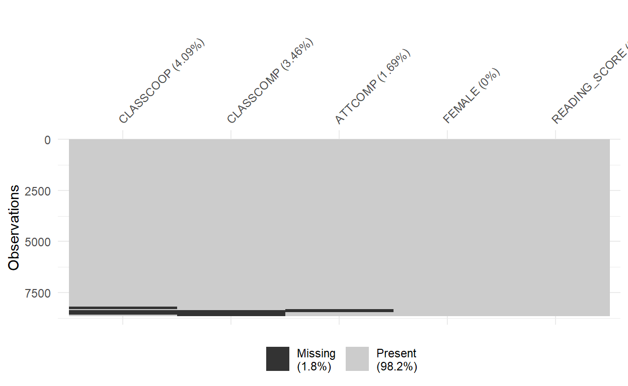
visdat::vis_miss(PISA_Subsetted, sort_miss = TRUE, cluster = TRUE)

Show code

naniar::gg_miss_upset(PISA_Subsetted, nsets = 5, nintersects = 10)

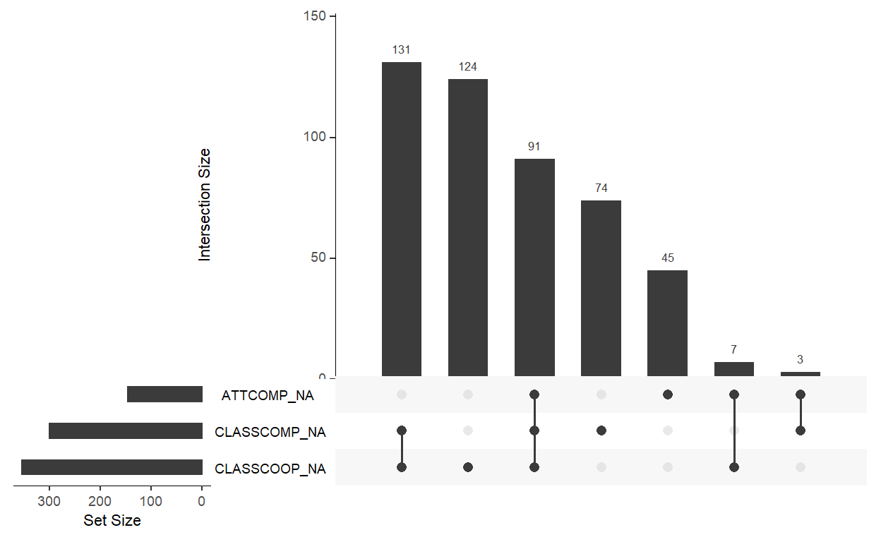
• It turns out we only have 1.8% of missing data. The missingness pattern indicates that the missing pair of perceived classroom cooperation and perceived classroom competition has the most frequency among all missing variables. There are also 91 cases that do not have any variable values. Given the discovered pattern, it makes more sense to remove them with listwise deletion instead of performing an imputation (aka plugging in possible numbers with an educated guess). Note that there is no rule of thumb in handling missing data. It depends on judgement of the researcher themselves. I tried imputing the data set as well and it gives no noticeable change, but I just want to try something different this time.

Show code

PISA_Subsetted <- na.omit(PISA_Subsetted)

Exploratory Data Analysis and Assumption Check

• To perform analyses using statistical learning, it is important to confirm that all statistical assumptions of the models were met to ensure that the results are meaningful. The assumptions that we will check in this section are normality distribution, multicollinearity, and influential outliers. There are other assumptions we need to check as well such as variable independence andhomoscedasticity (for the equality of variance throughout the data set), but we would have to create a linear regression model with the whole data set without teaching the machine. We won’t be doing that here because I aim to automate the process with the tidymodel approach instead of performing regression manually every time.

• We will first examine structure of the data set with plot_str to plot data structure and plot_intro to plot basic infornmation of the data set.

Show code

plot_intro(PISA_Subsetted, title = "Types of Variables")+
  theme(plot.title = element_text(hjust = 0.5))

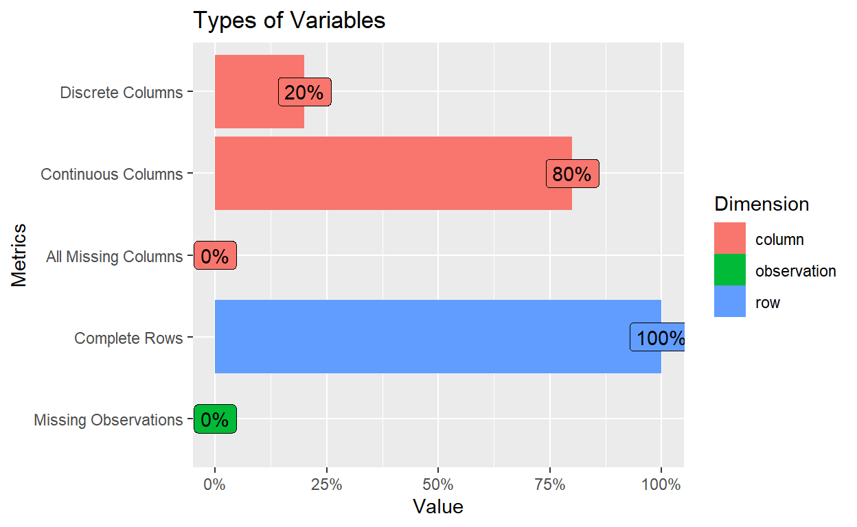
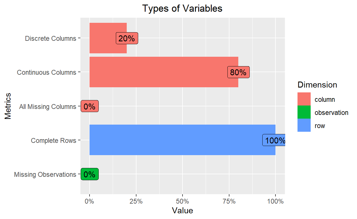
• This plot shows us how many discrete and continuous variables that we have in the data set. Mext, we will plot structure of the data to check which variable is numerical and which variable is factor.

Show code

plot_str(PISA_Subsetted)

• Next, we can check for normality distribution with histogram, skewness/kurtosis with descriptive statistics, and Quantile-Quantile Plot (Q-Q Plot).

Show code

describe(PISA_Subsetted)

              vars    n   mean    sd median trimmed   mad    min
FEMALE*          1 8158   1.46  0.50   1.00    1.45  0.00   1.00
READING_SCORE    2 8158 411.26 88.42 402.43  408.00 91.53 146.33
CLASSCOMP        3 8158   0.20  0.87   0.20    0.19  0.73  -1.99
CLASSCOOP        4 8158   0.20  0.92   0.60    0.22  1.07  -2.14
ATTCOMP          5 8158   0.03  0.79   0.20    0.00  0.65  -2.35
                 max  range  skew kurtosis   se
FEMALE*         2.00   1.00  0.18    -1.97 0.01
READING_SCORE 720.09 573.76  0.32    -0.37 0.98
CLASSCOMP       2.04   4.03  0.02    -0.04 0.01
CLASSCOOP       1.68   3.82 -0.39    -0.47 0.01
ATTCOMP         2.01   4.35  0.13     1.11 0.01

Show code

plot_histogram(PISA_Subsetted)

Show code

set.seed(123)
plot_qq(PISA_Subsetted, sampled_rows = 1000L)

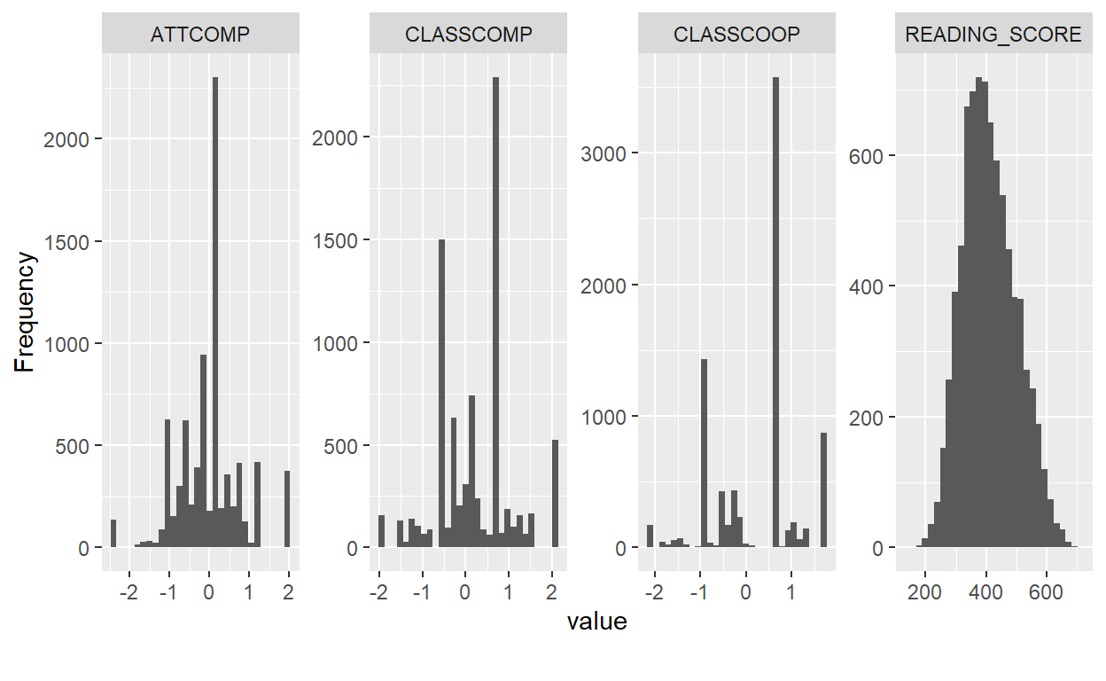
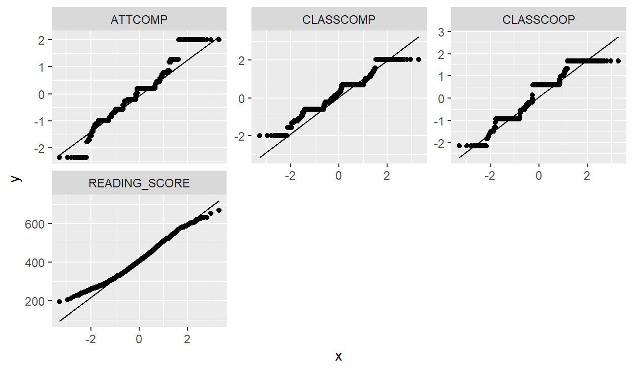
• The results of skewness and kurtosis indicate no departure from normality; that is, the data is normally distributed with all skewness stays between the range of -0.5 and 0.5, and all kurtosis stays between the range of -3 and 3 (Lomax and Hahs-Vaughn, 2012). The normality assumption is further confirmed with bell shape of the histogram and visualization from the Q-Q plots. Next, we will examine bivariate correlation between variables to investigate their relationships and confirm the absence of multicollinearity assumption.

• Multicollinearity refers to the condition where relationships between our variables of interest is high; this which may influence the result of our analysis because we are having two variables that investigate the same thing (Alin, 2010). For example, when you investigate the influence of person’s weight to their height and included both weight in pound and weight in kilogram, the results can be messed up because you include variables that measure to much of the same thing.

Show code

plot_correlation(PISA_Subsetted, type = "continuous", title = "Correlation Matrix") +
  theme(plot.title = element_text(hjust = 0.5))

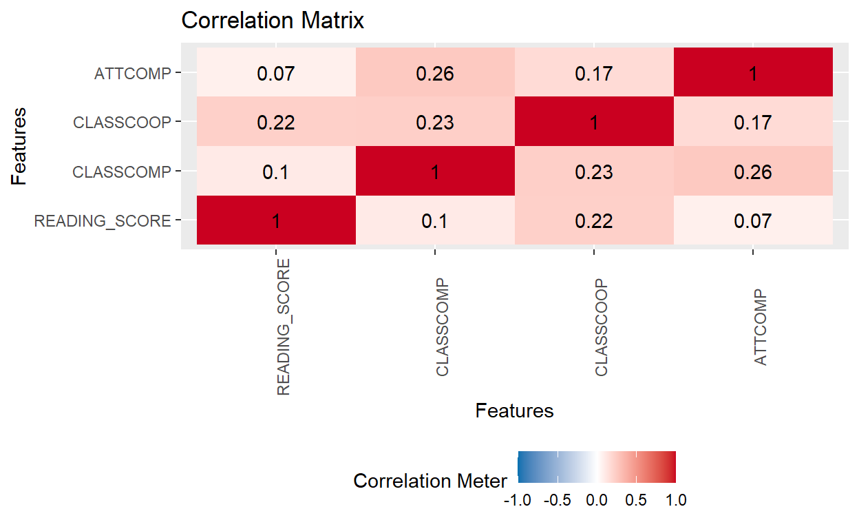
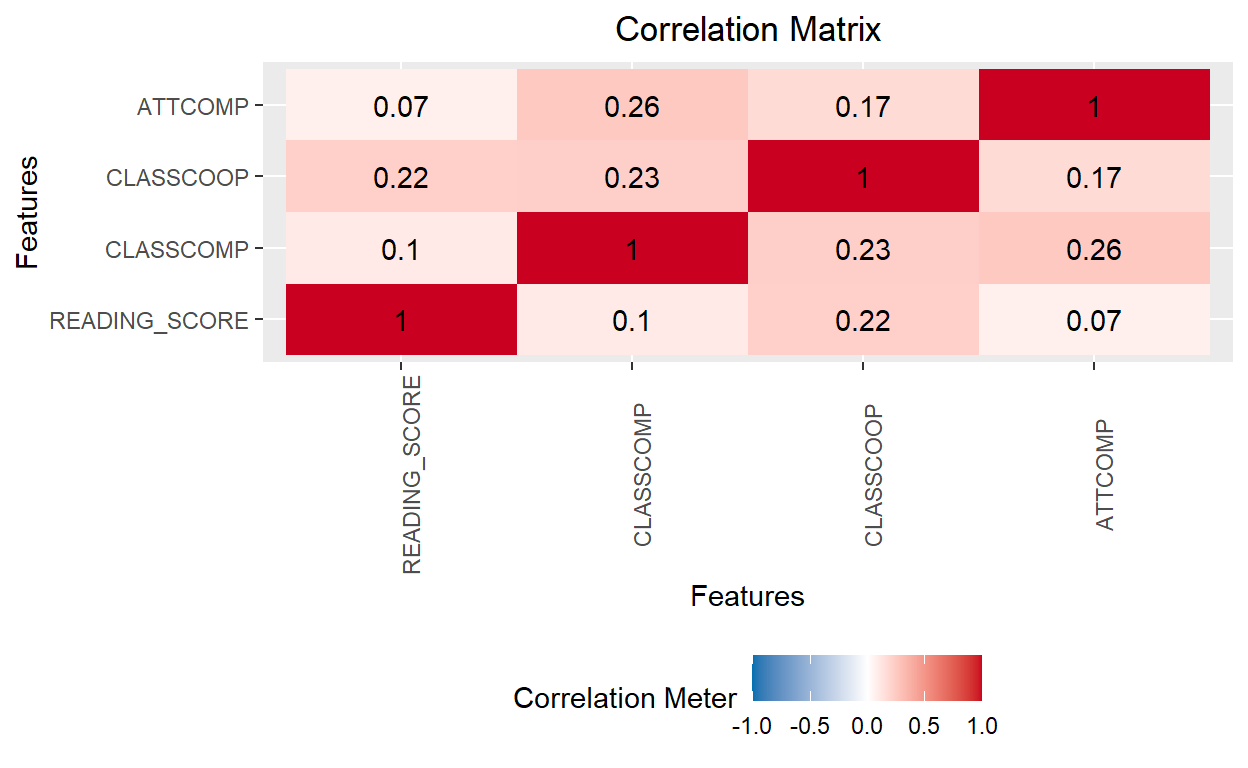
• All variables exhibit positive correlation to each other. The matrix shows no multicollinearity as the highest correlation coefficient between variables is 0.26, which is far from extreme in terms of magnitude (.6 to .7 coefficients should be flagged). For your reference, the report of data exploration can be generated with a simple function of create_report(PISA_Subsetted).

Data Preprocessing

• To test out our models, we need to split the data set into a training and a testing set to make sure that the testing is fair. It is similar to the situation where we do not want our students to take a peek at the exam before their test.

Show code

set.seed(456)

# Put 3/4 of the data into the training set 
data_split <- initial_split(PISA_Subsetted, prop = 3/4)

# Create data frames for the two sets:
train_data <- training(data_split) #3/4
test_data  <- testing(data_split)  #1/4

Linear Regression Model

• Now we have a training set that has 75% of the whole data and a testing set that has 25% of the whole data. Next, we will create a Linear Regression Model to predict the value of students’ reading score (READING_SCORE) with the degree of classroom cooperation, the degree of classroom competition, and students’ attitude to competition. First, we will request for a linear regression model with linear_reg() set the mode to regression and set the engine to “lm”, which stands for linear model.

Show code

lm_mod <- 
  linear_reg() %>% 
  set_mode("regression") %>%
  set_engine("lm")

lm_mod

Linear Regression Model Specification (regression)

Computational engine: lm 

• Next, we will do some data preprocessing by removing variables that we do not need in the analysis with recipe package. We will specify the formula as READING_SCORE ~ ., which means we will be predicting students’ reading score with all other variables. The step_rm() argument removes the variable we specified; for our case, it is students’ gender. For your reference, there are functions that assist us in other ways of data preprocessing as well such as step_dummy() to dummy code the variable or step_string2factor that converts string variables into factor variables.

Show code

PISA_linear_recipe <- 
  recipe(READING_SCORE ~ ., data = train_data) %>%
  step_rm(FEMALE)

PISA_linear_recipe

Recipe

Inputs:

      role #variables
   outcome          1
 predictor          4

Operations:

Variables removed FEMALE

• We have the model. We have the formula. Now, we can combine them both into a workflow with workflow()

Show code

PISA_workflow <- 
  workflow() %>% 
  add_model(lm_mod) %>% 
  add_recipe(PISA_linear_recipe)

PISA_workflow

== Workflow ==========================================================
Preprocessor: Recipe
Model: linear_reg()

-- Preprocessor ------------------------------------------------------
1 Recipe Step

* step_rm()

-- Model -------------------------------------------------------------
Linear Regression Model Specification (regression)

Computational engine: lm 

Fit the Linear Regression Model to the Training/Testing Dataset

• We will train (or teach) our Linear Regression model to learn characteristics of our data with the training set. This way, the machine will be able to predict values of the testing data with what it learned.

Show code

set.seed(678)

PISA_linear_fit <- 
  PISA_workflow %>% 
  fit(data = train_data)

• Now that we have taught the model, we can examine its performance by comparing its predicted value with the actual value of our targeted variable (i.e., students’ reading score). We will try extracting coefficients of the model first.

Show code

PISA_linear_fit %>% 
  extract_fit_parsnip() %>% 
  broom::tidy()

# A tibble: 4 x 5
  term        estimate std.error statistic  p.value
  <chr>          <dbl>     <dbl>     <dbl>    <dbl>
1 (Intercept)   406.        1.15    355.   0       
2 CLASSCOMP       3.77      1.33      2.84 4.50e- 3
3 CLASSCOOP      19.7       1.23     16.0  1.91e-56
4 ATTCOMP         3.08      1.45      2.12 3.38e- 2

• Coefficient interpretation is actually the same as interpreting linear regression results. First, we look at the p-value to see if any of these predictors are significant. Then, we interpret the coefficient of each prtedictor to the targeted variable. For example, the coefficient of 19.77 for the classroom cooperation variable means that every one-unit increase in the degree of classroom cooperation, students’ score will increase by 19.7. Next, we can evaluate performance of the model by comparing the predicted value with the actual value, as well as extracting values that can summarize overall performance.

Show code

PISA_linear_train_pred <- 
  predict(PISA_linear_fit, train_data) %>% 
  bind_cols(train_data %>% select(READING_SCORE)) 

PISA_linear_train_pred

# A tibble: 6,118 x 2
   .pred READING_SCORE
   <dbl>         <dbl>
 1  427.          471.
 2  421.          239.
 3  451.          546.
 4  405.          248.
 5  407.          457.
 6  398.          491.
 7  389.          308.
 8  421.          320.
 9  394.          473.
10  404.          507.
# ... with 6,108 more rows

• The .pred column is the predicted value and the READING_SCORE column is the actual value. We can see that some predicted numbers are off from the actual number. Let us see overall performance of the model with Mean-Squared Error (MSE), Root Mean-Squared Error (RMSE), and R-Squared (R^2). The first two values indicate how poor our model performs, and the third value indicates how many percent of the variation of our targeted variable is explained by the model.

Show code

mse_vec <- function(truth, estimate, na_rm = TRUE, ...) {
  
  mse_impl <- function(truth, estimate) {
    mean((truth - estimate) ^ 2)
  }
  
  metric_vec_template(
    metric_impl = mse_impl,
    truth = truth, 
    estimate = estimate,
    na_rm = na_rm,
    cls = "numeric",
    ...
  )
  
}

Show code

mse_vec(
  truth = PISA_linear_train_pred$READING_SCORE, 
  estimate = PISA_linear_train_pred$.pred
)

[1] 7389.577

Show code

rmse(PISA_linear_train_pred, 
     truth = READING_SCORE,
     estimate = .pred)

# A tibble: 1 x 3
  .metric .estimator .estimate
  <chr>   <chr>          <dbl>
1 rmse    standard        86.0

Show code

rsq(PISA_linear_train_pred, 
     truth = READING_SCORE,
     estimate = .pred)

# A tibble: 1 x 3
  .metric .estimator .estimate
  <chr>   <chr>          <dbl>
1 rsq     standard      0.0499

• We have MSE = 7389.577, RMSE = 86, and R-Squared = 0.0499 (or 4% of the targeted variable). Let us to the same for the testing round to ‘test’ out how well our model can predict the targeted variable.

Show code

PISA_linear_test_pred <- 
  predict(PISA_linear_fit, test_data) %>% 
  bind_cols(test_data %>% select(READING_SCORE)) 

PISA_linear_test_pred

# A tibble: 2,040 x 2
   .pred READING_SCORE
   <dbl>         <dbl>
 1  398.          477.
 2  427.          542.
 3  415.          519.
 4  422.          597.
 5  421.          467.
 6  434.          573.
 7  397.          522.
 8  425.          436.
 9  423.          440.
10  399.          543.
# ... with 2,030 more rows

Show code

mse_vec(
  truth = PISA_linear_test_pred$READING_SCORE, 
  estimate = PISA_linear_test_pred$.pred
)

[1] 7472.221

Show code

rmse(PISA_linear_test_pred, 
     truth = READING_SCORE,
     estimate = .pred)

# A tibble: 1 x 3
  .metric .estimator .estimate
  <chr>   <chr>          <dbl>
1 rmse    standard        86.4

Show code

rsq(PISA_linear_test_pred, 
     truth = READING_SCORE,
     estimate = .pred)

# A tibble: 1 x 3
  .metric .estimator .estimate
  <chr>   <chr>          <dbl>
1 rsq     standard      0.0584

• In the testing round, We have MSE = 7472.221, RMSE = 86.4, and R-Squared = 0.0584 (or 5% of the targeted variable). The performance of both training and testing round are similar, meaning that there is no overfit (the machine memorized its lesson too much / too strict) or underfit (the machine did not learn as much as it is supposed to and therefore unable to know the relationship between variables). Now that we know what Linear Regression can do, let us see what can we accomplish with Polynomial Regression.

Polynomial Regression Model

• Polynomial Regression is similar to Linear Regression, with the difference in its ability to capture non-linear relationship like the picture below. This ability allows the model to drop its assumption that the relationship between the independent and dependent variables has to be in linear shape.

Image from https://towardsdatascience.com/polynomial-regression-an-alternative-for-neural-networks-c4bd30fa6cf6. No copyright infringement is intended

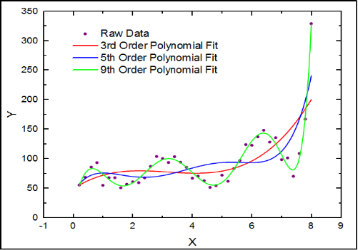
• We can customize ability to which our model can capture the pattern of our data by increasing its degree as demonstrated by the picture above. We can see that the red line (3rd degree) misses to capture a lot of patterns while the blue line (5th degree) captures a fair amount of patterns while the green line travels to almost every possible patterns. However, it is not necessarily true that the model with the highest degree is the best since it could capture noises that will not appear in the new data we will test the machine on (as well as the real-world data).

• So, after all we have discussed so far, let’s try creating a 3rd degree polynomial regression to see if we can capture the relationship any better than our linear regression. We will include step_poly with degree = 3 into the recipe function to make our model able to capture a degree of non-linearity.

Show code

PISA_poly_recipe <- 
  recipe(READING_SCORE ~ CLASSCOMP + CLASSCOOP + ATTCOMP, data = train_data) %>%
  step_poly(CLASSCOMP, degree = 3) %>%
  step_poly(CLASSCOOP, degree = 3)

PISA_poly_recipe

Recipe

Inputs:

      role #variables
   outcome          1
 predictor          3

Operations:

Orthogonal polynomials on CLASSCOMP
Orthogonal polynomials on CLASSCOOP

• Then, we will add the 3rd degree polynomial recipe to a workflow using the same model as our linear regression part (lm_mod).

Show code

PISA_poly_wf <- workflow() %>%
  add_model(lm_mod) %>%
  add_recipe(PISA_poly_recipe)

PISA_poly_wf

== Workflow ==========================================================
Preprocessor: Recipe
Model: linear_reg()

-- Preprocessor ------------------------------------------------------
2 Recipe Steps

* step_poly()
* step_poly()

-- Model -------------------------------------------------------------
Linear Regression Model Specification (regression)

Computational engine: lm 

• Finally, we can fit our model to the training data to teach it to recognize patterns of our training data set before using it to predict the testing data. While we are at it, we can use extract_fit_parsnip() to extract coefficients of our model as well to see which polynomial degree of which variable is significant in capturing patterns of the training data.

Show code

set.seed(999)

PISA_poly_fit <- 
  PISA_poly_wf %>%
  fit(data = train_data)

PISA_poly_fit

== Workflow [trained] ================================================
Preprocessor: Recipe
Model: linear_reg()

-- Preprocessor ------------------------------------------------------
2 Recipe Steps

* step_poly()
* step_poly()

-- Model -------------------------------------------------------------

Call:
stats::lm(formula = ..y ~ ., data = data)

Coefficients:
     (Intercept)           ATTCOMP  CLASSCOMP_poly_1  
         411.053             2.729           271.369  
CLASSCOMP_poly_2  CLASSCOMP_poly_3  CLASSCOOP_poly_1  
         295.526            19.960          1400.633  
CLASSCOOP_poly_2  CLASSCOOP_poly_3  
         -55.306           304.765  

Show code

PISA_poly_fit %>% 
  extract_fit_parsnip() %>% 
  broom::tidy()

# A tibble: 8 x 5
  term             estimate std.error statistic  p.value
  <chr>               <dbl>     <dbl>     <dbl>    <dbl>
1 (Intercept)        411.        1.10   374.    0       
2 ATTCOMP              2.73      1.45     1.88  6.00e- 2
3 CLASSCOMP_poly_1   271.       90.4      3.00  2.69e- 3
4 CLASSCOMP_poly_2   296.       88.4      3.34  8.31e- 4
5 CLASSCOMP_poly_3    20.0      87.2      0.229 8.19e- 1
6 CLASSCOOP_poly_1  1401.       88.7     15.8   4.97e-55
7 CLASSCOOP_poly_2   -55.3      88.6     -0.625 5.32e- 1
8 CLASSCOOP_poly_3   305.       87.2      3.50  4.75e- 4

• After we trained our model, we can use it to predict the unseen test data and compare it with our actual data to assess its accuracy.

Show code

PISA_poly_pred <- 
  predict(PISA_poly_fit, test_data) %>% 
  bind_cols(test_data %>% select(READING_SCORE)) 

kbl(head(PISA_poly_pred)) %>%
  kable_styling(bootstrap_options = c("striped", "hover", "condensed", "responsive"),
                full_width = TRUE, position = "left")  

.pred	READING_SCORE
398.7327	476.744
426.4006	542.238
410.2957	518.744
417.5398	597.441
415.7663	466.964
431.5449	572.923

• To check if our 3rd degree polynomial model performed well, we can extract MSE, RMSE, and R^2 as our performance metrics.

Show code

mse_vec(
  truth = PISA_poly_pred$READING_SCORE, 
  estimate = PISA_poly_pred$.pred)

[1] 7470.233

Show code

rmse(PISA_poly_pred, 
     truth = READING_SCORE,
     estimate = .pred)

# A tibble: 1 x 3
  .metric .estimator .estimate
  <chr>   <chr>          <dbl>
1 rmse    standard        86.4

Show code

rsq(PISA_poly_pred, 
     truth = READING_SCORE,
     estimate = .pred)

# A tibble: 1 x 3
  .metric .estimator .estimate
  <chr>   <chr>          <dbl>
1 rsq     standard      0.0584

• The metrics show that our polynomial slightly outperform our linear regression model, with higher R-squared and lower MSE. The problem is, how do we know if 3rd degree is the most appropriate degree we can make to predict our data. For polynomial regression, we can look for the most appropriate polynomial degree via cross-validation.

Model Tuning with Cross Validation

• Cross-Validation is a way to evaluate performance of our machine learning models by dividing our data into smaller groups and use them to estimate how the model will perform in when used to make predictions on data that are not in our training set. Basically, we test our machines with smaller tests to see which of them qualifies for the final test. Another way we can see this is when we tune an old ratio to make it able to receive the clearest frequency of the broadcast, but we use the machines to automatically do it instead to save our time and effort.

• We will begin by setting up our recipe with tune() and add it to a workflow.

Show code

PISA_poly_tuned_recipe <- 
  recipe(READING_SCORE ~ CLASSCOMP + CLASSCOOP + ATTCOMP, data = train_data) %>%
  step_poly(CLASSCOMP, CLASSCOOP, degree = tune())

PISA_poly_wf <- workflow() %>%
  add_model(lm_mod) %>%
  add_recipe(PISA_poly_tuned_recipe)

PISA_poly_wf

== Workflow ==========================================================
Preprocessor: Recipe
Model: linear_reg()

-- Preprocessor ------------------------------------------------------
1 Recipe Step

* step_poly()

-- Model -------------------------------------------------------------
Linear Regression Model Specification (regression)

Computational engine: lm 

• Then, we will create smaller data sets from our training set. We will create 10 sets (or 10 folds) to test 10 candidates of our model, which are models with polynomial degree from 1 (equivalent to linear regression), 2 (quadratic regression), 3 (cubic regression),…, to 10 (decic regression). In other words, we are looking for the model that performs the best among 10 candidates using RMSE and R-Squared as our performance metrics.

Show code

train_data_subsetted = subset(train_data, select = c('READING_SCORE','CLASSCOMP','CLASSCOOP','ATTCOMP'))

PISA_folds <- vfold_cv(train_data, v = 10)

degree_grid <- grid_regular(degree(range = c(1, 10)), levels = 10)

tune_resample <- tune_grid(
  object = PISA_poly_wf, 
  resamples = PISA_folds, 
  grid = degree_grid)

autoplot(tune_resample)

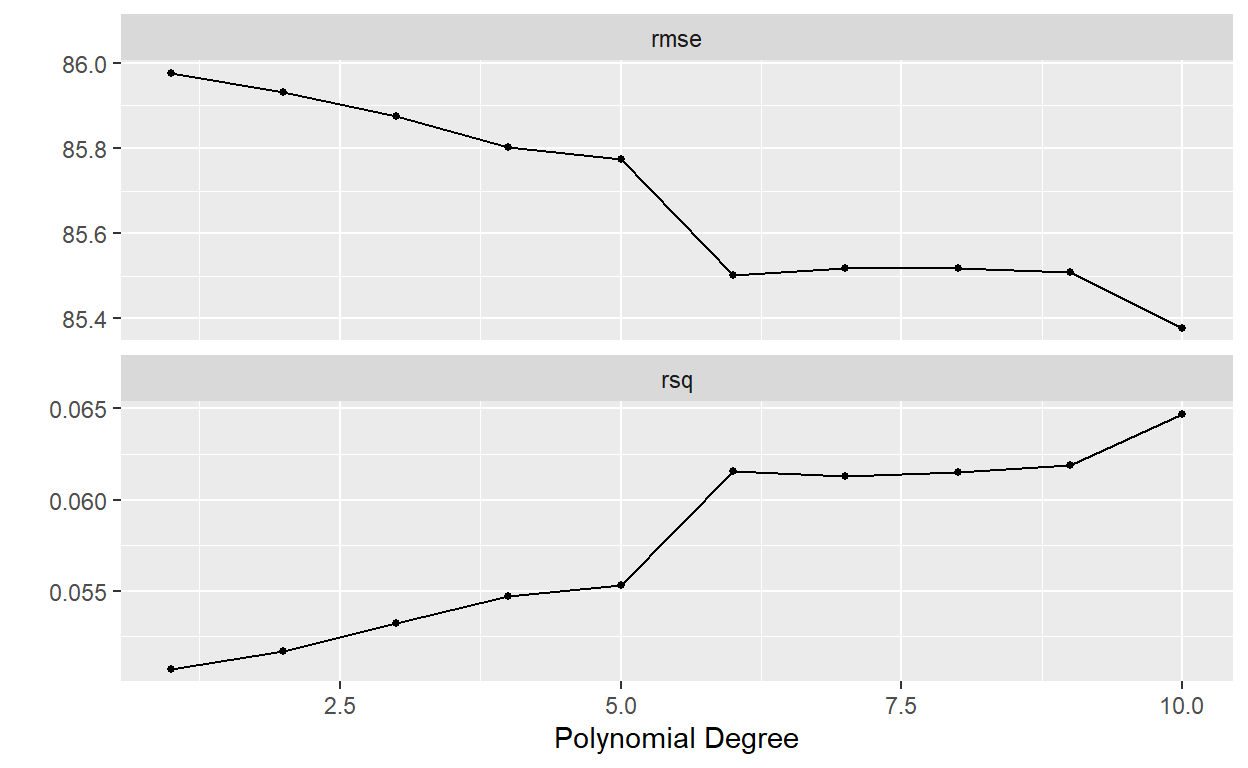
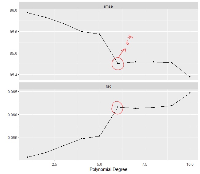
• We want RMSE to be as low as possible and R-Squared to be as high as possible. However, our models can only do so much. Their performance will remain somewhat steady when it reaches a certain point. In our case, it is from the 6th polynomial degree onward. While the plot suggests that the 10th polynomial degree performed the best, we do not want our model to be too complex as it can be harder to interpret. We want the model that performs the best and is easiest to interpret. For that, we might want to pick the model that comes right after a significant performance boost to not make it too complex while able to bring out its maximum performance, which is the 6th degree polynomial model (Sextic Regression).

Data Tuning Results with 10-Folds Cross Validation

• To dive into the numbers, we can have the software shows and selects the best model candidate to include it in our final model.

Show code

show_best(tune_resample, metric = "rmse")

# A tibble: 5 x 7
  degree .metric .estimator  mean     n std_err .config              
   <dbl> <chr>   <chr>      <dbl> <int>   <dbl> <chr>                
1     10 rmse    standard    85.4    10   0.852 Preprocessor10_Model1
2      6 rmse    standard    85.5    10   0.845 Preprocessor06_Model1
3      9 rmse    standard    85.5    10   0.860 Preprocessor09_Model1
4      8 rmse    standard    85.5    10   0.857 Preprocessor08_Model1
5      7 rmse    standard    85.5    10   0.843 Preprocessor07_Model1

Show code

select_by_one_std_err(tune_resample, degree, metric = "rsq")

# A tibble: 1 x 9
  degree .metric .estimator   mean     n std_err .config  .best .bound
   <dbl> <chr>   <chr>       <dbl> <int>   <dbl> <chr>    <dbl>  <dbl>
1      6 rsq     standard   0.0616    10 0.00730 Prepro~ 0.0647 0.0563

Final Model

• We will then assign the best model candidate as our best_degree to include it in the final workflow. Then, as usual, we teach (fit) it and test it with our test data.

Show code

best_degree <- select_by_one_std_err(tune_resample, degree, metric = "rsq")

final_wf <- finalize_workflow(PISA_poly_wf, best_degree)

final_fit <- fit(final_wf, train_data)

final_fit

== Workflow [trained] ================================================
Preprocessor: Recipe
Model: linear_reg()

-- Preprocessor ------------------------------------------------------
1 Recipe Step

* step_poly()

-- Model -------------------------------------------------------------

Call:
stats::lm(formula = ..y ~ ., data = data)

Coefficients:
     (Intercept)           ATTCOMP  CLASSCOMP_poly_1  
         411.050             2.836           279.070  
CLASSCOMP_poly_2  CLASSCOMP_poly_3  CLASSCOMP_poly_4  
         300.125            19.260          -167.827  
CLASSCOMP_poly_5  CLASSCOMP_poly_6  CLASSCOOP_poly_1  
        -197.978          -477.187          1381.076  
CLASSCOOP_poly_2  CLASSCOOP_poly_3  CLASSCOOP_poly_4  
         -56.933           281.590          -251.840  
CLASSCOOP_poly_5  CLASSCOOP_poly_6  
        -130.564           389.358  

• Now, we will test our model and extract its performance metrics to evaluate it.

Show code

PISA_poly_test_pred <- 
  predict(final_fit, test_data) %>% 
  bind_cols(test_data %>% select(READING_SCORE))

mse_vec(
  truth = PISA_poly_test_pred$READING_SCORE, 
  estimate = PISA_poly_test_pred$.pred)

[1] 7382.151

Show code

rmse(PISA_poly_test_pred, 
     truth = READING_SCORE,
     estimate = .pred)

# A tibble: 1 x 3
  .metric .estimator .estimate
  <chr>   <chr>          <dbl>
1 rmse    standard        85.9

Show code

rsq(PISA_poly_test_pred, 
     truth = READING_SCORE,
     estimate = .pred)

# A tibble: 1 x 3
  .metric .estimator .estimate
  <chr>   <chr>          <dbl>
1 rsq     standard      0.0697

• To compare the performance of both Linear Regression and 6th Degree Polynomial Regression, we will create a comparison table to compare their performance for our discussion.

Show code

tabl <- "
| Model         | R-Square      | MSE   | RMSE |
|---------------|:-------------:|------:|-----:|
| Linear Reg    | 0.0584        | 7472.2| 86.4 |
| Sextic Reg    | 0.0697        | 7382.1| 85.9 |
"
cat(tabl)

Model	R-Square	MSE	RMSE
Linear Reg	0.0584	7472.2	86.4
Sextic Reg	0.0697	7382.1	85.9

• The table shows that our sextic regression slightly outperform our linear regression model as seen from its higher R-Squared and Lower Error Value (i.e., MSE, RMSE).

Final Remarks and Conclusion

• What we have done so far is developing two predictive models of linear regression and polynomial regression to predict students’ reading score from the degree of classroom cooperation, the degree of classroom competition, and students’ attitude to competition. While the traditional statistical approach examines the entire data set to make retrospective inferences, the statistical learning approach that we use both examines the relationship between the predictors and the targeted variables as well as testing predictive power of our models with the hold-out testing set, so that it can be used with new data we may receive in the future.

• However, considering the differences in performance metrics between the two algorithm, linear regression could be more appropriate with the variables examined in this study as its performance is slightly lower than sextic Regression at the trade-off of model interpretability. In other words, it is easier to interpret the model to non-technical audience and therefore easier to put the result into practice.

• We can incorporate the model into an early warning system to inform teachers in their feedback provision to students in addition to other information such as students’ score and their class history. However, note that the models we developed in this post is far from perfect. The data set used in this study is relatively outdated as the new data of PISA 2022 cycle will be released in the future. Performance of the models leaves much to be desired as only 6% of the dependent variable was accounted for at most.

• The thing is, we have accomplished what we are here for. We have tried our hands on developing a couple models with a large scale data set and user it to predict unseen data with statistical learning approach. Instead of going for complex models like Random Forest or Artificial Neural Networks, sticking to the ground with basic models could also be feasible in the actual practice as well. This is the point I am trying to make in this post. Thank you very much for reading. Have a good one!