Introduction
A lot of my recent posts are about supervised machine learning problems, which is defined by its use of labeled datasets to train algorithms to classify or predict outcomes of the unseen data set. In other words, the model was trained (or supervised) by humans to achieve the best possible predictive capability. However, unsupervised machine learning is defined in opposition to supervised learning. Unsupervised learning, in contrast, is learning without labels. It is pure pattern discovery, unguided by a prediction task. The model learns from raw data without any prior knowledge or human training.
For example, you have a group of customers with a variety of characteristics such as age, location, and financial history. You wish to discover patterns and sort them into natural “clusters” without tampering with them in any ways. Or perhaps you have a set of texts, such as Wikipedia pages, and you wish to segment them into categories based on their content. These are examples of unsupervised learning techniques called “clustering” and “dimension reduction”.
Unsupervised learning is called as such because you are not guiding the pattern discovery by some prediction task, but instead uncovering hidden structure from unlabeled data. In this post, I will be using two unsupervised learning techniques with a data set, namely K-means clustering and Hierarchical clustering, to determine groups of customers from their age, income, and spending behavior data. As usual, we will import the necessary modules first to set up the environment.
Show code
import numpy as np
import pandas as pd
import matplotlib.pyplot as plt
import seaborn as sns

from sklearn.cluster import KMeans
import scipy.cluster.hierarchy as sch
from sklearn.cluster import AgglomerativeClustering

import warnings
warnings.filterwarnings('ignore')
About the Data Set
- This data set is created by Kaggle for the learning purpose of the data segmentation concepts. The scenario is as follows: you are owning a supermarket mall. Through membership cards , you have some basic data about your customers like Customer ID, age, gender, annual income and spending score. Spending Score is something you assign to the customer based on your defined parameters like customer behavior and purchasing data. Specifically put, if you buy a lot, you get a lot of scores to be posted on a top spender board. Below is the information about the data set we will be using in this task.
Show code
df = pd.read_csv("customers.csv")

# data set shape
print("The data set has", df.shape[0], "cases and", df.shape[1], "variables")

# print head of data set
The data set has 200 cases and 5 variablesShow code
print(df.head(10)) CustomerID Gender Age Annual Income (k$) Spending Score (1-100)
0 1 1 19 15 39
1 2 1 21 15 81
2 3 0 20 16 6
3 4 0 23 16 77
4 5 0 31 17 40
5 6 0 22 17 76
6 7 0 35 18 6
7 8 0 23 18 94
8 9 1 64 19 3
9 10 0 30 19 72Show code
df.info()<class 'pandas.core.frame.DataFrame'>
RangeIndex: 200 entries, 0 to 199
Data columns (total 5 columns):
# Column Non-Null Count Dtype
--- ------ -------------- -----
0 CustomerID 200 non-null int64
1 Gender 200 non-null int64
2 Age 200 non-null int64
3 Annual Income (k$) 200 non-null int64
4 Spending Score (1-100) 200 non-null int64
dtypes: int64(5)
memory usage: 7.9 KBShow code
df.describe()

#Check for missing data
CustomerID Gender ... Annual Income (k$) Spending Score (1-100)
count 200.000000 200.000000 ... 200.000000 200.000000
mean 100.500000 0.440000 ... 60.560000 50.200000
std 57.879185 0.497633 ... 26.264721 25.823522
min 1.000000 0.000000 ... 15.000000 1.000000
25% 50.750000 0.000000 ... 41.500000 34.750000
50% 100.500000 0.000000 ... 61.500000 50.000000
75% 150.250000 1.000000 ... 78.000000 73.000000
max 200.000000 1.000000 ... 137.000000 99.000000
[8 rows x 5 columns]Show code
df.isnull().sum()CustomerID 0
Gender 0
Age 0
Annual Income (k$) 0
Spending Score (1-100) 0
dtype: int64- We will first begin by exploring distribution of the data set to examine if their distribution is normal. Then, we can examine the distribution of each variable pair as indicated by density plots and scatter plots. We will also examine correlation coefficients between all variables with a heatmap and potential clusters with a cluster map as well.
Show code
plt.figure(1 , figsize = (15 , 6))
n = 0
for x in ['Age' , 'Annual Income (k$)' , 'Spending Score (1-100)']:
    n += 1
    plt.subplot(1 , 3 , n)
    plt.subplots_adjust(hspace = 0.5 , wspace = 0.5)
    sns.distplot(df[x] , bins = 15)
    plt.title('Distplot of {}'.format(x))

plt.show()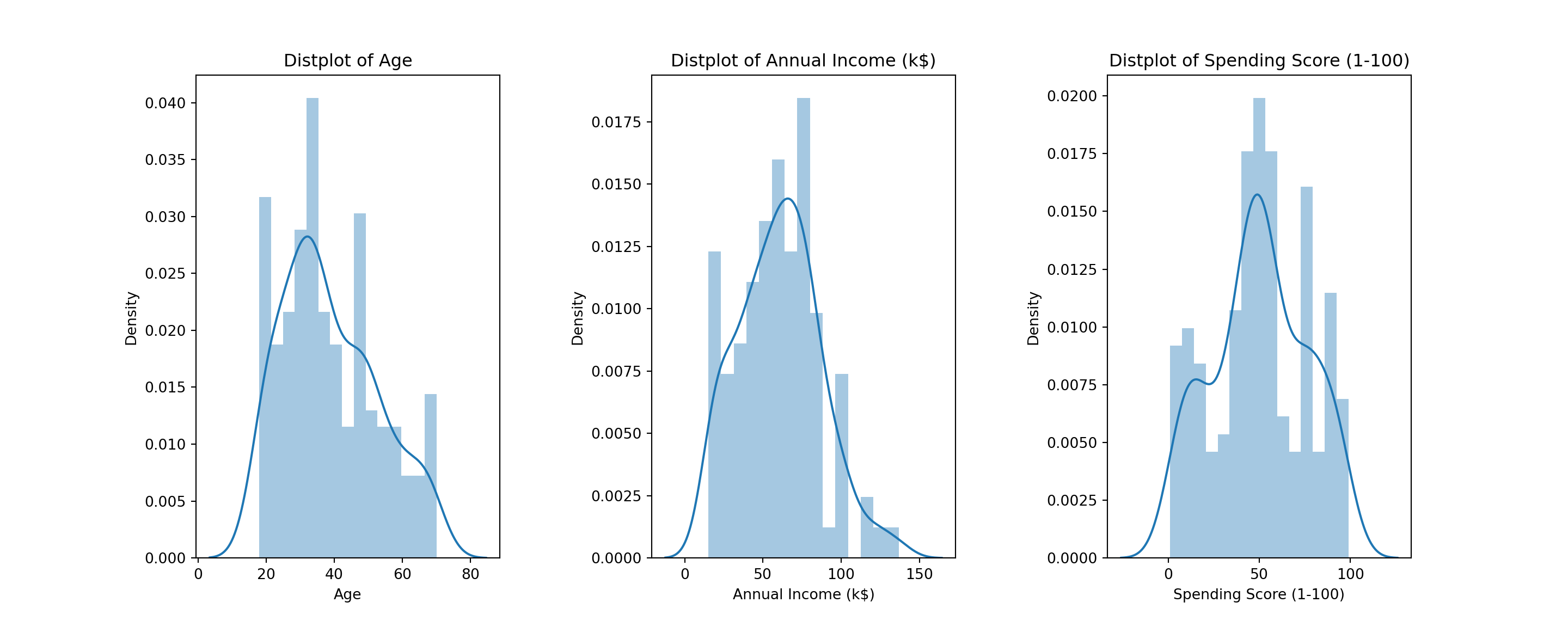
Show code
sns.heatmap(df.corr(), annot=True, cmap="YlGnBu")
plt.show()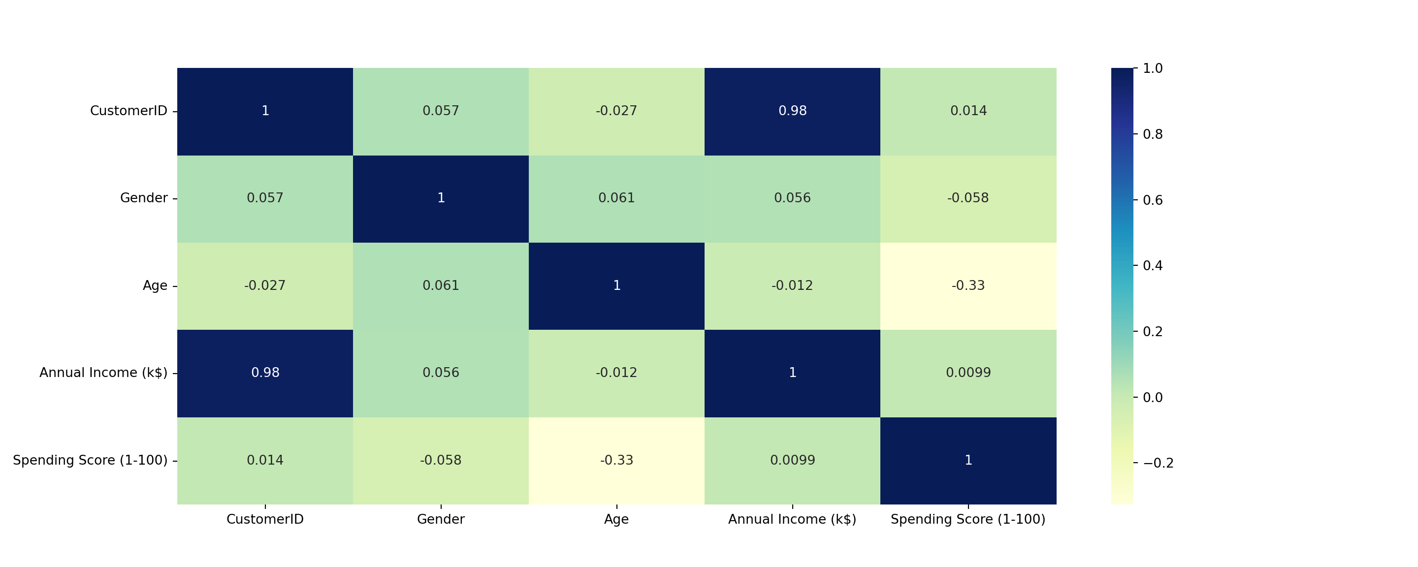
Show code
plt.figure(1, figsize = (16 ,8))
sns.clustermap(df)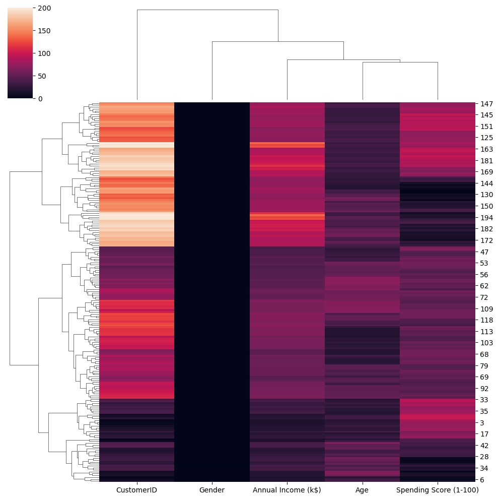
Show code
sns.pairplot(df, vars = ['Spending Score (1-100)', 'Annual Income (k$)', 'Age'], hue = "Gender")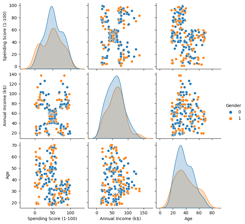
K-Means Clustering
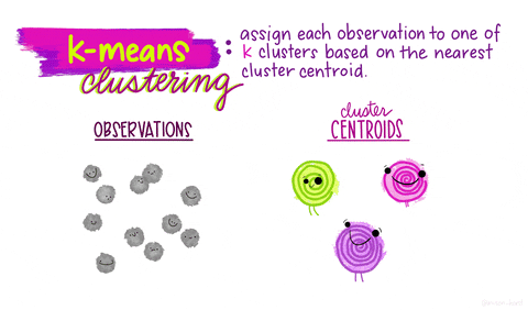
K-means clustering is one of the simplest and popular unsupervised machine learning algorithms. For this method, we define a target number k, which refers to the number of centroids you need in the dataset. A centroid is the imaginary or real location representing the center of the cluster; then, the algorithm allocates every data point to the nearest cluster, while keeping the centroids as small as possible. The means in the K-means refers to averaging of the data in finding their corresponding centroids.
Instead of using equations, this short animation by Allison Horst explains k-means clustering in a very cute and comprehensive way.
Show code
plt.figure(1 , figsize = (15 , 7))
plt.title('Scatter plot of Age v/s Spending Score', fontsize = 20)
plt.xlabel('Age')
plt.ylabel('Spending Score')
plt.scatter( x = 'Age', y = 'Spending Score (1-100)', data = df, s = 100)
plt.show()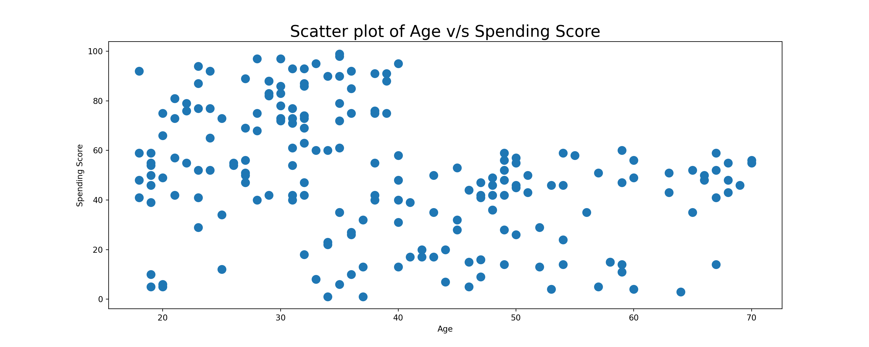
- Clustering is basically the process of mapping data points into classes of similar objects. The scatter plot above maps the relationship between customers’ age and their spending score. It could be challenging at this point to determine how many clusters can be seen in this 2D pane. This is where clustering comes into play. We will first examine how many clusters should we group the data points into with the elbow method. To find the optimal K for a dataset, we need to find the point where the decrease in inertia begins to slow. K=3 is the “elbow” of this graph, so the points after that are K=4 or K=5.
Show code
X1 = df[['Age' , 'Spending Score (1-100)']].iloc[: , :].values
inertia = []

for n in range(1 , 15):
    algorithm = (KMeans(n_clusters = n ,init='k-means++', n_init = 10 ,max_iter=300,
                        tol=0.0001,  random_state= 111  , algorithm='full') )
    algorithm.fit(X1)
    inertia.append(algorithm.inertia_)
KMeans(algorithm='full', n_clusters=1, random_state=111)
KMeans(algorithm='full', n_clusters=2, random_state=111)
KMeans(algorithm='full', n_clusters=3, random_state=111)
KMeans(algorithm='full', n_clusters=4, random_state=111)
KMeans(algorithm='full', n_clusters=5, random_state=111)
KMeans(algorithm='full', n_clusters=6, random_state=111)
KMeans(algorithm='full', n_clusters=7, random_state=111)
KMeans(algorithm='full', random_state=111)
KMeans(algorithm='full', n_clusters=9, random_state=111)
KMeans(algorithm='full', n_clusters=10, random_state=111)
KMeans(algorithm='full', n_clusters=11, random_state=111)
KMeans(algorithm='full', n_clusters=12, random_state=111)
KMeans(algorithm='full', n_clusters=13, random_state=111)
KMeans(algorithm='full', n_clusters=14, random_state=111)
Show code
plt.figure(1 , figsize = (15 ,6))
plt.plot(np.arange(1 , 15) , inertia , 'o')
plt.plot(np.arange(1 , 15) , inertia , '-' , alpha = 0.5)
plt.xlabel('Number of Clusters') , plt.ylabel('Inertia')
(Text(0.5, 0, 'Number of Clusters'), Text(0, 0.5, 'Inertia'))Show code
plt.show()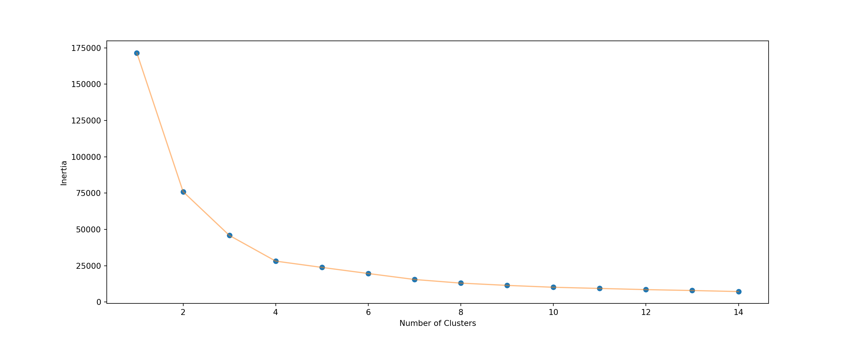
- The elbow plot shows that grouping the data into 4 or 5 clusters seems to be the best as the inertia, which measures how well a dataset was clustered by K-Means, seems to reach the optimal point at 4 and 5 clusters. A good model is the one with low inertia AND a low number of clusters (K). However, this is a tradeoff because as K increases, inertia decreases. We want the inertia to be as low as possible, but we don’t want to have 12+ clusters as well (I mean, why would you group your data anyway if you want it to have a lot of clusters). We can try clustering the data into 4 clusters first, then we can go with 5 later.
Show code
algorithm = (KMeans(n_clusters = 4 ,init='k-means++', n_init = 10 ,max_iter=300,
                        tol=0.0001,  random_state= 111  , algorithm='full') )
algorithm.fit(X1)
KMeans(algorithm='full', n_clusters=4, random_state=111)Show code
labels1 = algorithm.labels_
centroids1 = algorithm.cluster_centers_

h = 0.02
x_min, x_max = X1[:, 0].min() - 1, X1[:, 0].max() + 1
y_min, y_max = X1[:, 1].min() - 1, X1[:, 1].max() + 1
xx, yy = np.meshgrid(np.arange(x_min, x_max, h), np.arange(y_min, y_max, h))
Z = algorithm.predict(np.c_[xx.ravel(), yy.ravel()])

plt.figure(1 , figsize = (15 , 7) )
plt.clf()
Z = Z.reshape(xx.shape)
plt.imshow(Z , interpolation='nearest',
           extent=(xx.min(), xx.max(), yy.min(), yy.max()),
           cmap = plt.cm.Pastel2, aspect = 'auto', origin='lower')

plt.scatter( x = 'Age', y = 'Spending Score (1-100)', data = df, c = labels1, s = 100)
plt.scatter(x = centroids1[: , 0] , y =  centroids1[: , 1] , s = 300 , c = 'red' , alpha = 0.5)
plt.ylabel('Spending Score (1-100)') , plt.xlabel('Age')
(Text(0, 0.5, 'Spending Score (1-100)'), Text(0.5, 0, 'Age'))Show code
plt.title("Four Clusters", loc='center')
plt.show() 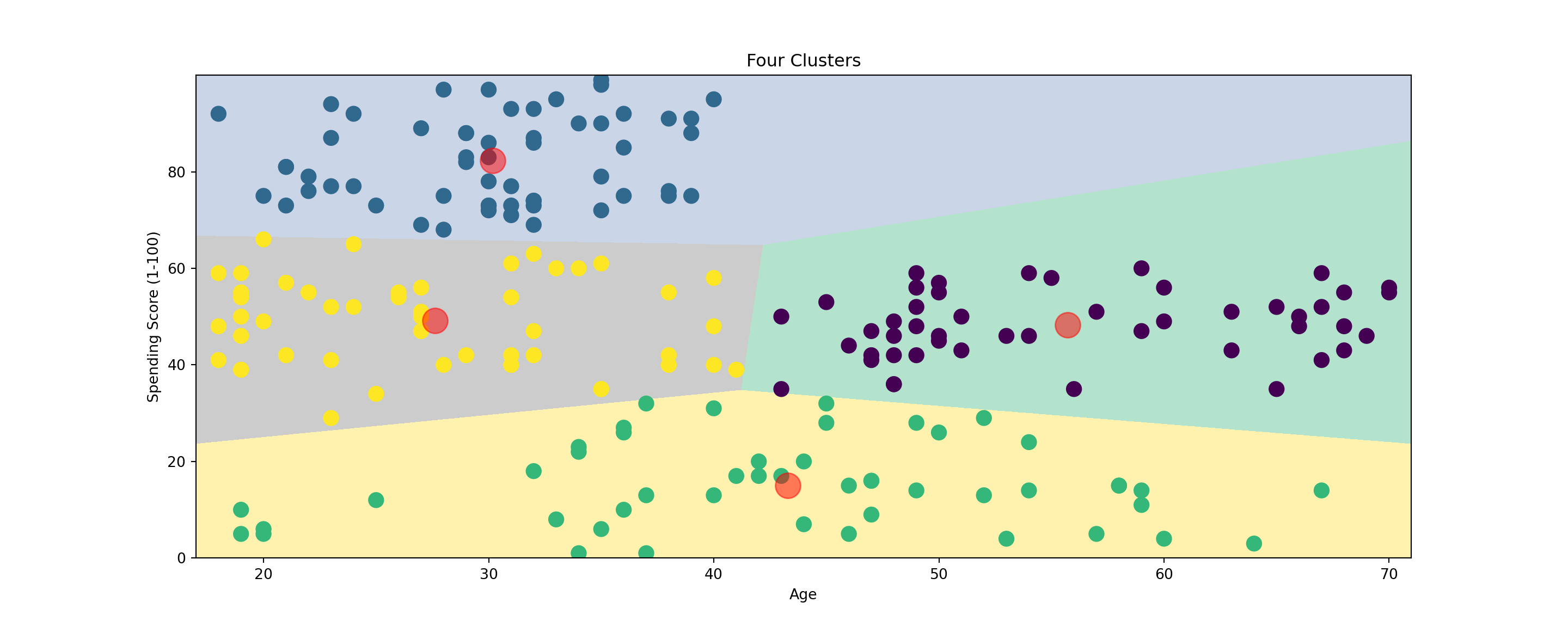
Show code
#%%Applying KMeans for k=5

algorithm = (KMeans(n_clusters = 5, init='k-means++', n_init = 10, max_iter=300,
                        tol=0.0001, random_state= 111 , algorithm='elkan'))
algorithm.fit(X1)
KMeans(algorithm='elkan', n_clusters=5, random_state=111)Show code
labels1 = algorithm.labels_
centroids1 = algorithm.cluster_centers_

h = 0.02
x_min, x_max = X1[:, 0].min() - 1, X1[:, 0].max() + 1
y_min, y_max = X1[:, 1].min() - 1, X1[:, 1].max() + 1
xx, yy = np.meshgrid(np.arange(x_min, x_max, h), np.arange(y_min, y_max, h))
Z = algorithm.predict(np.c_[xx.ravel(), yy.ravel()])

plt.figure(1 , figsize = (15 , 7) )
plt.clf()
Z = Z.reshape(xx.shape)
plt.imshow(Z , interpolation='nearest',
           extent=(xx.min(), xx.max(), yy.min(), yy.max()),
           cmap = plt.cm.Pastel2, aspect = 'auto', origin='lower')

plt.scatter( x = 'Age', y = 'Spending Score (1-100)', data = df, c = labels1, s = 100)
plt.scatter(x = centroids1[: , 0] , y =  centroids1[: , 1] , s = 300 , c = 'red' , alpha = 0.5)
plt.ylabel('Spending Score (1-100)') , plt.xlabel('Age')
(Text(0, 0.5, 'Spending Score (1-100)'), Text(0.5, 0, 'Age'))Show code
plt.title("Five Clusters", loc='center')
plt.show()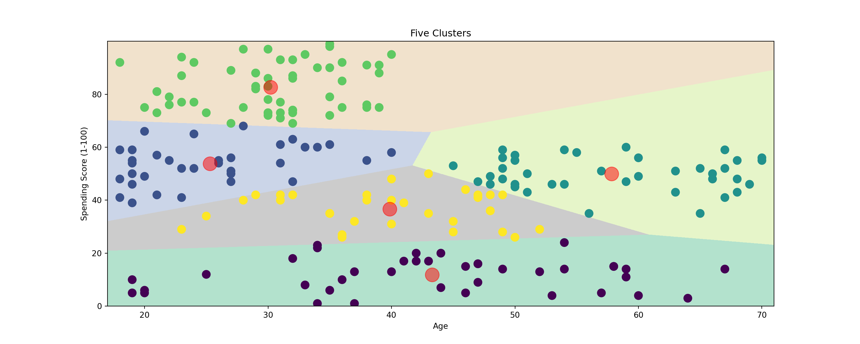
The two diagrams above show what it is like when we group the data into 4 and 5 clusters. It is important that the clusters are stable. Even though the algorithm begins by randomly initializing the cluster centers, if the k-means algorithm is the right choice for the data, then different runs of the algorithm will result in similar clusters in terms of size and variable distribution. If there is a lot of change in clusters between the different iterations of the algorithm, then k-means clustering may not be the right choice for the data. However, it is not possible to validate that the clusters obtained from the algorithm are accurate because there is no patient labeling; thus, it is necessary to examine how the clusters change between different iterations of the algorithm and check if the number of clusters makes sense in both theoretical and practical sense. We can also have domain experts give their opinions about if the clusters of customer make practical sense.
For one more practice, we can try making a cluster based on annual income and spending score.
Show code
X2 = df[['Annual Income (k$)' , 'Spending Score (1-100)']].iloc[: , :].values
inertia = []
for n in range(1 , 11):
    algorithm = (KMeans(n_clusters = n ,init='k-means++', n_init = 10 ,max_iter=300,
                        tol=0.0001,  random_state= 111  , algorithm='full') )
    algorithm.fit(X2)
    inertia.append(algorithm.inertia_)
KMeans(algorithm='full', n_clusters=1, random_state=111)
KMeans(algorithm='full', n_clusters=2, random_state=111)
KMeans(algorithm='full', n_clusters=3, random_state=111)
KMeans(algorithm='full', n_clusters=4, random_state=111)
KMeans(algorithm='full', n_clusters=5, random_state=111)
KMeans(algorithm='full', n_clusters=6, random_state=111)
KMeans(algorithm='full', n_clusters=7, random_state=111)
KMeans(algorithm='full', random_state=111)
KMeans(algorithm='full', n_clusters=9, random_state=111)
KMeans(algorithm='full', n_clusters=10, random_state=111)
Show code
plt.figure(1 , figsize = (15 ,6))
plt.plot(np.arange(1 , 11) , inertia , 'o')
plt.plot(np.arange(1 , 11) , inertia , '-' , alpha = 0.5)
plt.xlabel('Number of Clusters') , plt.ylabel('Inertia')
(Text(0.5, 0, 'Number of Clusters'), Text(0, 0.5, 'Inertia'))Show code
plt.show()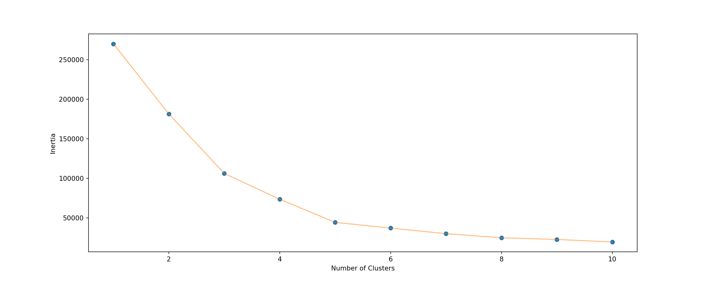
Show code
algorithm = (KMeans(n_clusters = 5 ,init='k-means++', n_init = 10 ,max_iter=300,
                        tol=0.0001,  random_state= 111  , algorithm='elkan') )
algorithm.fit(X2)
KMeans(algorithm='elkan', n_clusters=5, random_state=111)Show code
labels2 = algorithm.labels_
centroids2 = algorithm.cluster_centers_

#%%
h = 0.02
x_min, x_max = X2[:, 0].min() - 1, X2[:, 0].max() + 1
y_min, y_max = X2[:, 1].min() - 1, X2[:, 1].max() + 1
xx, yy = np.meshgrid(np.arange(x_min, x_max, h), np.arange(y_min, y_max, h))
Z2 = algorithm.predict(np.c_[xx.ravel(), yy.ravel()])


#%%

plt.figure(1 , figsize = (15 , 7) )
plt.clf()
Z2 = Z2.reshape(xx.shape)
plt.imshow(Z2 , interpolation='nearest',
           extent=(xx.min(), xx.max(), yy.min(), yy.max()),
           cmap = plt.cm.Pastel2, aspect = 'auto', origin='lower')

plt.scatter( x = 'Annual Income (k$)' ,y = 'Spending Score (1-100)' , data = df , c = labels2 ,
            s = 100 )
plt.scatter(x = centroids2[: , 0] , y =  centroids2[: , 1] , s = 300 , c = 'red' , alpha = 0.5)
plt.ylabel('Spending Score (1-100)') , plt.xlabel('Annual Income (k$)')
(Text(0, 0.5, 'Spending Score (1-100)'), Text(0.5, 0, 'Annual Income (k$)'))Show code
plt.title("Five Clusters", loc='center')
plt.show()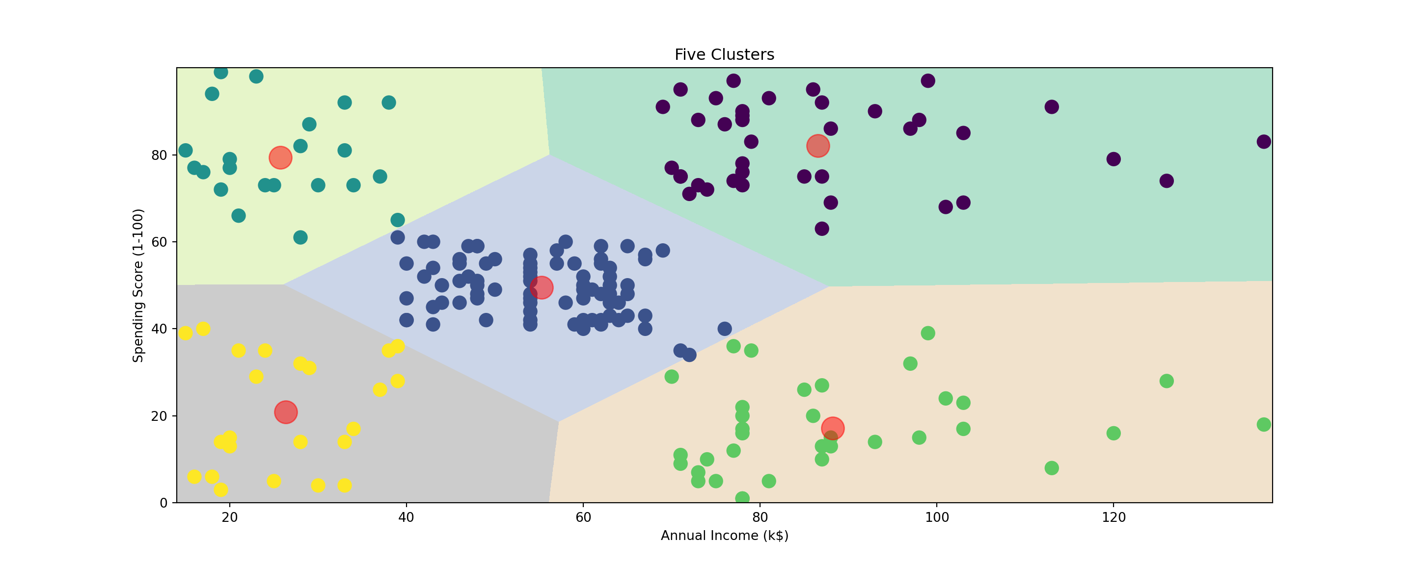
Hierarchical Clustering
An alternative to k-means clustering is hierarchical clustering (also known as hierarchical cluster analysis), which groups similar objects into hierarchies (or levels) of clusters. The end product is a set of clusters, where each cluster is distinct on its own, and the objects within each cluster are broadly similar to each other. This method works well when data have a nested structure - meaning that one characteristic is related to another (e.g., spending habit of a certain age group).
Again, Allison Horst did a really good job explaining how hierarchical clustering works with her visuals below. Note that the visual is for the “single” method, but we will be using the “ward” method. However, they are similar in terms of how they build a hierarchical dendrogram. A dendrogram is a diagram representing a tree that, in this context, illustrates the arrangement of the clusters produced by the corresponding analyses.
We will try performing divisive hierarchical clustering first. This method is known as a top-down approach that splits a cluster that contains the whole data into smaller clusters recursively until each single data point have been splitted into singleton clusters or the termination condition holds. This method is rigid. Once a merging or splitting is done, it can never be undone.
Show code
plt.figure(1, figsize = (16 ,8))
dendrogram = sch.dendrogram(sch.linkage(df, method  = "ward"))

plt.title('Dendrogram')
plt.xlabel('Customers')
plt.ylabel('Euclidean distances')
plt.show()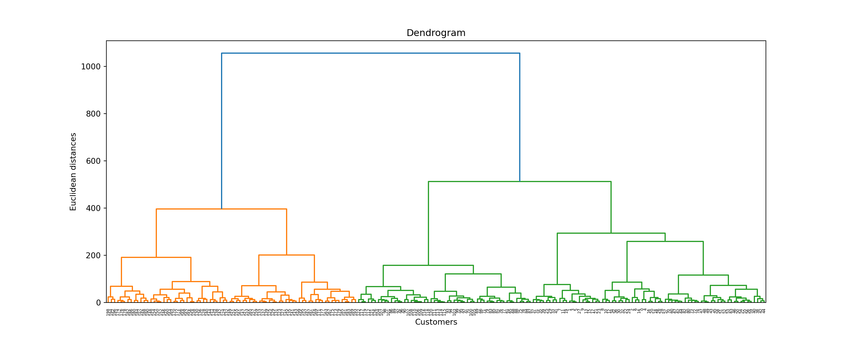
- Next, we will try agglomerative clustering. This method is known as a “bottom-up” approach; that is, each observation starts in its own cluster, and pairs of clusters are merged as one amd moved up the hierarchy. We start with each object forming a separate group. It keeps on merging the objects or groups that are close to one another. The iteration keeps on doing so until all of the groups are merged into one or until the termination condition holds.
Show code
hc = AgglomerativeClustering(n_clusters = 5, affinity = 'euclidean', linkage ='average')

y_hc = hc.fit_predict(df)
y_hc
array([3, 4, 3, 4, 3, 4, 3, 4, 3, 4, 3, 4, 3, 4, 3, 4, 3, 4, 3, 4, 3, 4,
3, 4, 3, 4, 3, 4, 3, 4, 3, 4, 3, 4, 3, 4, 3, 4, 3, 4, 3, 4, 3, 2,
3, 2, 2, 2, 2, 2, 2, 2, 2, 2, 2, 2, 2, 2, 2, 2, 2, 2, 2, 2, 2, 2,
2, 2, 2, 2, 2, 2, 2, 2, 2, 2, 2, 2, 2, 2, 2, 2, 2, 2, 2, 2, 2, 2,
2, 2, 2, 2, 2, 2, 2, 2, 2, 2, 2, 2, 2, 2, 2, 2, 2, 2, 2, 2, 2, 2,
2, 2, 2, 2, 2, 2, 2, 2, 2, 2, 2, 2, 2, 1, 0, 1, 2, 1, 0, 1, 0, 1,
0, 1, 0, 1, 0, 1, 0, 1, 0, 1, 0, 1, 0, 1, 0, 1, 0, 1, 0, 1, 0, 1,
0, 1, 0, 1, 0, 1, 0, 1, 0, 1, 0, 1, 0, 1, 0, 1, 0, 1, 0, 1, 0, 1,
0, 1, 0, 1, 0, 1, 0, 1, 0, 1, 0, 1, 0, 1, 0, 1, 0, 1, 0, 1, 0, 1,
0, 1], dtype=int64)Show code
X = df.iloc[:, [3,4]].values
plt.scatter(X[y_hc==0, 0], X[y_hc==0, 1], s=100, c='red', label ='Cluster 1')
plt.scatter(X[y_hc==1, 0], X[y_hc==1, 1], s=100, c='blue', label ='Cluster 2')
plt.scatter(X[y_hc==2, 0], X[y_hc==2, 1], s=100, c='green', label ='Cluster 3')
plt.scatter(X[y_hc==3, 0], X[y_hc==3, 1], s=100, c='purple', label ='Cluster 4')
plt.scatter(X[y_hc==4, 0], X[y_hc==4, 1], s=100, c='orange', label ='Cluster 5')
plt.title('Clusters of Customers (Hierarchical Clustering Model)')
plt.xlabel('Annual Income(k$)')
plt.ylabel('Spending Score(1-100)')
plt.show()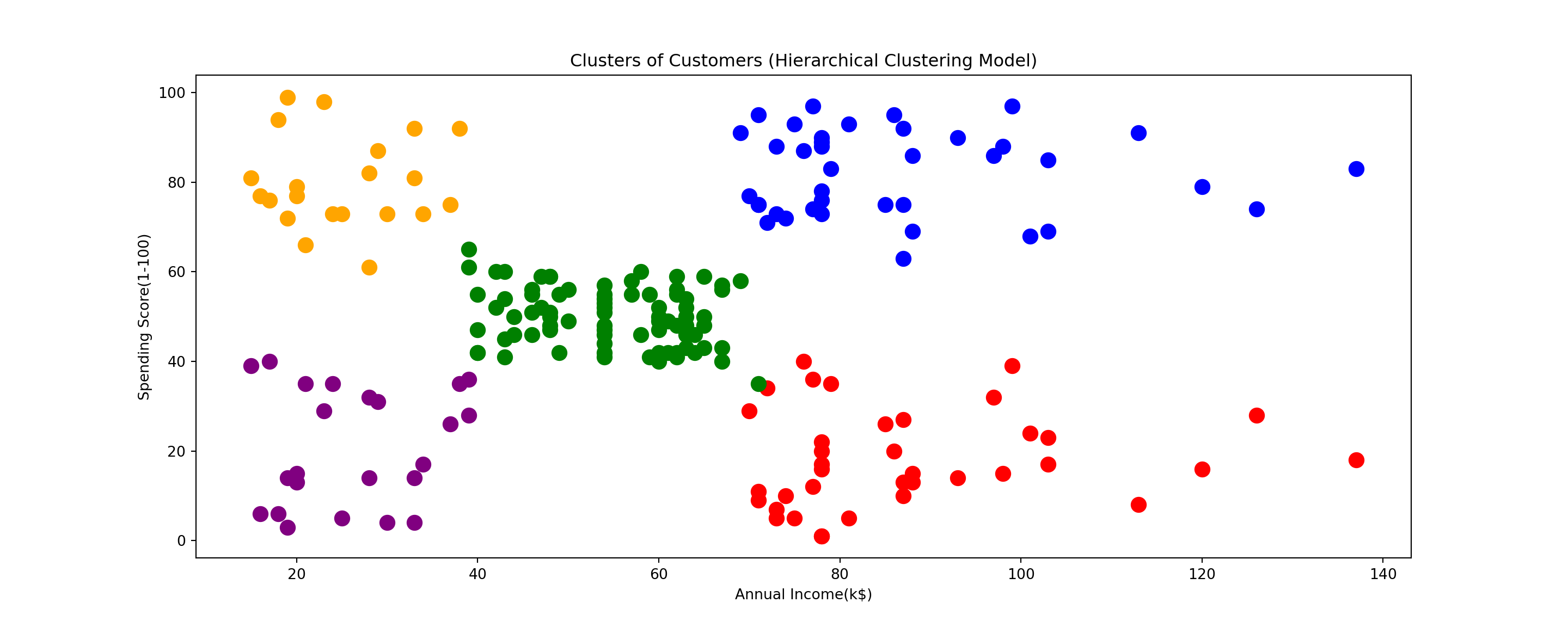
Conclusion
- The main advantage of clustering over classification is that it is adaptable to changes and helps single out useful features that distinguish different groups. This is a useful tool for data scientists to understand raw data with unsupervised learning. The methods is best used for exploratory purposes for applications such as the investigation of a group that stands out the most and identify useful features that affect them. Specifically, The method can be used to discover distinct groups in their customer base, categorize genes with similar functionality, gain insight into structures inherent to populations in Biology, or even classify documents on the web for information discovery by combining clustering with natural language processing techniques. As always, thank you very much for reading this!