Introduction
Hi, Everyone. It’s been really hot here in Summer. I have some more time before my next school year (2023) begins. As I learned more about Psychometric, I came to know about techniques that can be used to reduce the number of questions in a questionnaire for efficiency. This post was inspired by my supervisor’s post of the same technique. He applied the data to the Experiences in Close Relationships (ECR) scale of Adult Romantic Attachment Measure (Brennan et al., 1998). I want to try following his footstep and replicate the same techniques to a different data set for my practice. In this post, I will use Genetic Algorithm and Ant Colony Optimization Algorithm to automatically shorten the length of a test.
We will be using the International Personality Item Pool data set (Goldberg et al., 2006). The data set has polytomous test items; that is, answers from test takers can be more than two values. Instead of “right” and “wrong”, the answer can be “strongly disagree”, “disagree”, “neutral”, “agree”, and “strongly agree”. The test measures person’s characteristics of extraversion, emotional stability, agreeableness, conscientiousness, and openness to experience.
First, we will import the data set and subset a portion of the data for feasibility. The full data set has 176,380 cases. We will subset only 5000 of them.
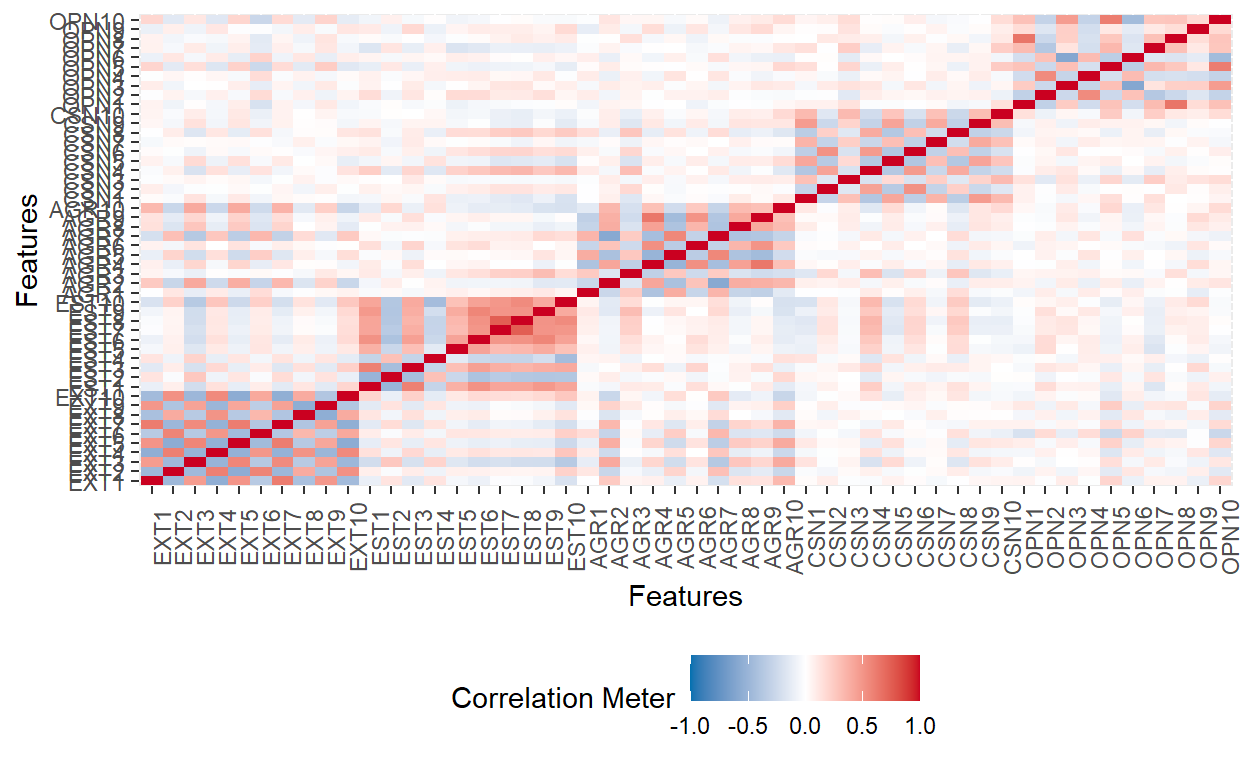
- The data set contains responses of individuals to 50 personality test questions. Each response is on ordinal scale, meaning that the response can be categorized and ranked (i.e., disagree - neutral - agree). The correlation plot below indicates relationships between items measuring the same dimension (e.g., extraversion). Items with negative correlation are reverse-coded, meaning that the items are rephrased to have an opposite meaning. For example, a question measuring extraversion may ask “I see myself as someone who is talkative”. The reverse-coded version maybe “I see myself as someone who tends to be quiet”.
Show code
df_survey <- df[1:5000, 1:50]

head(df_survey)
   EXT1 EXT2 EXT3 EXT4 EXT5 EXT6 EXT7 EXT8 EXT9 EXT10 EST1 EST2 EST3
1:    4    1    5    2    5    1    5    2    4     1    1    4    4
2:    3    5    3    4    3    3    2    5    1     5    2    3    4
3:    2    3    4    4    3    2    1    3    2     5    4    4    4
4:    2    2    2    3    4    2    2    4    1     4    3    3    3
5:    3    3    3    3    5    3    3    5    3     4    1    5    5
6:    3    3    4    2    4    2    2    3    3     4    3    4    3
   EST4 EST5 EST6 EST7 EST8 EST9 EST10 AGR1 AGR2 AGR3 AGR4 AGR5 AGR6
1:    2    2    2    2    2    3     2    2    5    2    4    2    3
2:    1    3    1    2    1    3     1    1    4    1    5    1    5
3:    2    2    2    2    2    1     3    1    4    1    4    2    4
4:    2    3    2    2    2    4     3    2    4    3    4    2    4
5:    3    1    1    1    1    3     2    1    5    1    5    1    3
6:    2    2    1    2    1    2     2    2    3    1    4    2    3
   AGR7 AGR8 AGR9 AGR10 CSN1 CSN2 CSN3 CSN4 CSN5 CSN6 CSN7 CSN8 CSN9
1:    2    4    3     4    3    4    3    2    2    4    4    2    4
2:    3    4    5     3    3    2    5    3    3    1    3    3    5
3:    1    4    4     3    4    2    2    2    3    3    4    2    4
4:    2    4    3     4    2    4    4    4    1    2    2    3    1
5:    1    5    5     3    5    1    5    1    3    1    5    1    5
6:    2    3    4     4    3    2    4    1    3    2    4    3    4
   CSN10 OPN1 OPN2 OPN3 OPN4 OPN5 OPN6 OPN7 OPN8 OPN9 OPN10
1:     4    5    1    4    1    4    1    5    3    4     5
2:     3    1    2    4    2    3    1    4    2    5     3
3:     2    5    1    2    1    4    2    5    3    4     4
4:     4    4    2    5    2    3    1    4    4    3     3
5:     5    5    1    5    1    5    1    5    3    5     5
6:     3    5    1    5    1    3    1    5    4    5     2
Show code
DataExplorer::plot_correlation(df_survey)
- The test has 10 items (or questions) in each domain, totalling 50
test items. This number seems reasonable, but we could further reduce
the number of items to avoid fatiguing our examinee. One way we can
reduce the number is through the use of coefficient alpha reliability.
The
alphafunction inpsychpackage can be used to examine how much reliability the test will have after dropping some items.
Show code
alpha <- psych::alpha(df_survey, check.keys=TRUE)
alpha$alpha.drop
       raw_alpha std.alpha   G6(smc) average_r      S/N    alpha se
EXT1-  0.8696207 0.8679394 0.9137837 0.1182655 6.572282 0.002611411
EXT2   0.8691535 0.8675726 0.9134115 0.1179326 6.551309 0.002621739
EXT3-  0.8668282 0.8651111 0.9121684 0.1157390 6.413506 0.002671484
EXT4   0.8683708 0.8667878 0.9129267 0.1172256 6.506819 0.002638125
EXT5-  0.8673617 0.8656936 0.9123513 0.1162518 6.445660 0.002659426
EXT6   0.8685602 0.8667696 0.9132939 0.1172093 6.505797 0.002632815
EXT7-  0.8682855 0.8668348 0.9129689 0.1172677 6.509470 0.002640926
EXT8   0.8712934 0.8695949 0.9150056 0.1197881 6.668412 0.002577510
EXT9-  0.8704641 0.8687061 0.9143138 0.1189665 6.616502 0.002593862
EXT10  0.8683898 0.8669061 0.9133637 0.1173317 6.513491 0.002638721
EST1   0.8703855 0.8687731 0.9141121 0.1190281 6.620390 0.002594302
EST2-  0.8715179 0.8698555 0.9152856 0.1200308 6.683770 0.002572223
EST3   0.8713890 0.8698611 0.9149559 0.1200360 6.684096 0.002575067
EST4-  0.8722369 0.8705305 0.9161060 0.1206634 6.723826 0.002558568
EST5   0.8712487 0.8695326 0.9155456 0.1197302 6.664750 0.002576908
EST6   0.8697921 0.8682577 0.9140230 0.1185557 6.590577 0.002606440
EST7   0.8698114 0.8682822 0.9134175 0.1185780 6.591988 0.002605601
EST8   0.8695089 0.8680298 0.9130377 0.1183477 6.577465 0.002612008
EST9   0.8692737 0.8677100 0.9136737 0.1180571 6.559153 0.002617047
EST10  0.8680675 0.8667208 0.9130501 0.1171656 6.503046 0.002644521
AGR1   0.8729617 0.8708241 0.9162004 0.1209403 6.741382 0.002540781
AGR2-  0.8696206 0.8674465 0.9136713 0.1178184 6.544122 0.002609287
AGR3   0.8720020 0.8701186 0.9156558 0.1202767 6.699333 0.002559864
AGR4-  0.8718810 0.8699519 0.9145632 0.1201208 6.689461 0.002561684
AGR5   0.8713817 0.8694433 0.9147959 0.1196472 6.659506 0.002572622
AGR6-  0.8740795 0.8722052 0.9166081 0.1222577 6.825042 0.002520054
AGR7   0.8695310 0.8674391 0.9132795 0.1178118 6.543703 0.002610839
AGR8-  0.8712084 0.8692263 0.9151725 0.1194462 6.646796 0.002576807
AGR9-  0.8719947 0.8700279 0.9149316 0.1201919 6.693960 0.002559508
AGR10- 0.8692295 0.8669770 0.9138922 0.1173954 6.517496 0.002617962
CSN1-  0.8715010 0.8696873 0.9151554 0.1198740 6.673849 0.002569307
CSN2   0.8743915 0.8722266 0.9165440 0.1222783 6.826354 0.002512017
CSN3-  0.8729250 0.8712122 0.9165431 0.1213081 6.764712 0.002542491
CSN4   0.8695425 0.8679183 0.9139521 0.1182463 6.571073 0.002609660
CSN5-  0.8713024 0.8695137 0.9151010 0.1197126 6.663639 0.002573481
CSN6   0.8723390 0.8703796 0.9153758 0.1205215 6.714834 0.002551467
CSN7-  0.8739940 0.8724664 0.9170480 0.1225097 6.841070 0.002522233
CSN8   0.8704663 0.8686382 0.9148756 0.1189042 6.612566 0.002591175
CSN9-  0.8724726 0.8705899 0.9156435 0.1207194 6.727375 0.002550163
CSN10- 0.8718644 0.8699681 0.9157181 0.1201359 6.690420 0.002563072
OPN1-  0.8731489 0.8713227 0.9152167 0.1214131 6.771378 0.002536994
OPN2   0.8723907 0.8704576 0.9152106 0.1205948 6.719479 0.002551733
OPN3-  0.8742745 0.8725471 0.9161203 0.1225876 6.846034 0.002516526
OPN4   0.8733534 0.8715435 0.9160396 0.1216236 6.784738 0.002533974
OPN5-  0.8710467 0.8687933 0.9141883 0.1190467 6.621561 0.002579241
OPN6   0.8723086 0.8703180 0.9150081 0.1204637 6.711173 0.002553227
OPN7-  0.8718728 0.8699217 0.9156417 0.1200926 6.687679 0.002563265
OPN8-  0.8752372 0.8730645 0.9163104 0.1230898 6.878014 0.002497109
OPN9   0.8760793 0.8755095 0.9191497 0.1255113 7.032742 0.002491151
OPN10- 0.8716998 0.8695968 0.9144305 0.1197899 6.668526 0.002565750
            var.r      med.r
EXT1-  0.02247896 0.08151262
EXT2   0.02242356 0.08166635
EXT3-  0.02239961 0.07907977
EXT4   0.02233050 0.08041782
EXT5-  0.02230091 0.07914325
EXT6   0.02288756 0.07930301
EXT7-  0.02235567 0.08146699
EXT8   0.02281218 0.08201026
EXT9-  0.02271017 0.08153477
EXT10  0.02258192 0.08041782
EST1   0.02257745 0.08146699
EST2-  0.02293955 0.08210536
EST3   0.02261406 0.08151262
EST4-  0.02326988 0.08180150
EST5   0.02327337 0.08157208
EST6   0.02262279 0.08082590
EST7   0.02258286 0.08146699
EST8   0.02248911 0.08132409
EST9   0.02280470 0.08041782
EST10  0.02268410 0.08002237
AGR1   0.02320503 0.08201026
AGR2-  0.02287127 0.08108114
AGR3   0.02323923 0.08151262
AGR4-  0.02249784 0.08225522
AGR5   0.02279661 0.08201026
AGR6-  0.02261039 0.08321513
AGR7   0.02275238 0.08092384
AGR8-  0.02309551 0.08162526
AGR9-  0.02265465 0.08180150
AGR10- 0.02322872 0.07874079
CSN1-  0.02314059 0.08166635
CSN2   0.02285444 0.08249577
CSN3-  0.02337612 0.08195375
CSN4   0.02299208 0.08082590
CSN5-  0.02315868 0.08157208
CSN6   0.02302597 0.08225522
CSN7-  0.02294173 0.08385676
CSN8   0.02335693 0.07998131
CSN9-  0.02305508 0.08195375
CSN10- 0.02344565 0.08162526
OPN1-  0.02302069 0.08295971
OPN2   0.02315918 0.08201026
OPN3-  0.02266237 0.08249577
OPN4   0.02310353 0.08225522
OPN5-  0.02321234 0.08082590
OPN6   0.02315973 0.08201026
OPN7-  0.02343876 0.08146699
OPN8-  0.02269568 0.08336518
OPN9   0.02248538 0.08407870
OPN10- 0.02292938 0.08162526
Show code
summary(alpha)
Reliability analysis
 raw_alpha std.alpha G6(smc) average_r S/N    ase mean   sd median_r
      0.87      0.87    0.92      0.12 6.8 0.0025  2.7 0.44    0.082
Genetic Algorithm
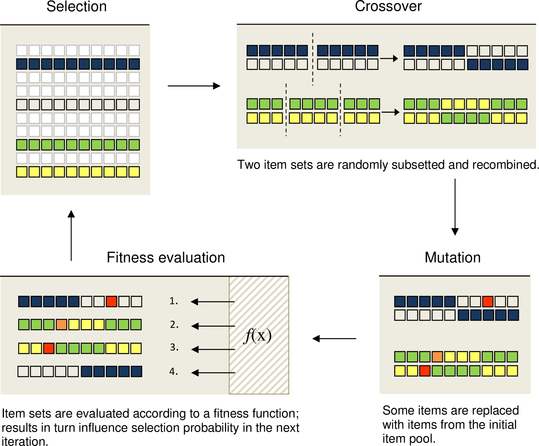
Another way we can reduce the number of items is through the use of Genetic Algorithm, which is an optimization method inspired from the natural selection theory (Schroeders et al., 2016). This is how it works:
First, the algorithm randomly selects several item sets from the item pool. These item sets act as parents.
Second, the algorithm picks items from each parent to form several sets of items as children (or an offspring).
Third, some items in the children set were exchanged with items from the item pool as a mutation.
Fourth, the children were evaluated. Children who produce better results were kept while those that did not do well are discarded. The process continues until a certain criterion is met.
Figure 1 below from visualizes how the process is done.
- We will use the
GAabbreviatepackage to perform test abbreviation with the Genetic Algorithm (Sahdra et al., 2016). To prepare the data, we will first create summations of scores in each domain for every examinee as the scale score. We will also transform the data frame into a matrix.
Show code
library(GAabbreviate)

scales = cbind(rowSums(df_survey[, 1:10]),
               rowSums(df_survey[, 11:20]),
               rowSums(df_survey[, 21:30]),
               rowSums(df_survey[, 31:40]),
               rowSums(df_survey[, 41:50]))

df_survey <- as.data.frame(sapply(df_survey, as.integer))

df_survey <- matrix(as.integer(unlist(df_survey)), nrow=nrow(df_survey))
- We will create the Genetic Algorithm object with the
GAabbreviatefunction (Sahdra et al, 2016). We will set the cost of each item to 0.001 so that the algorithm can produce results that explains the most variance (Yarkoni, 2010).
Show code
ipip_ga <- GAabbreviate(items = df_survey, # Matrix of item responses
                      verbose = FALSE,
                      scales = scales, # Scale scores
                      itemCost = 0.001, # The cost of each item
                      maxItems = 5, # Max number of items per dimension
                      maxiter = 1000, # Max number of iterations
                      run = 100, # Number of runs
                      crossVal = TRUE, # Cross-validation
                      seed = RANDOM_STATE) # Seed for reproducibility
- We can request for a summary of the algorithm below. The algorithm ran 301 times before achieving the best results. The number of items in the final set is 25, meaning that we reduced the test in half.
Show code
summary(ipip_ga)
── Genetic Algorithm ───────────────────

GA settings:
Type                  =  binary
Population size       =  50
Number of generations =  1000
Elitism               =  2
Crossover probability =  0.8
Mutation probability  =  0.1

GA results:
Iterations             = 301
Total cost             = 1.74582
Number of items in initial set = 50
Number of items in final set = 25
Mean coefficient alpha = 0.3212
Mean convergent correlation (training) = 0.8069
Mean convergent correlation (validation) = 0.8029- We can call for coefficient alpha reliability of the test dimensions below. Reliability of the emotional stability, agreeableness, and openness to experience dimension are satisfactory (0.80 for emotional stability, 0.73 for agreeableness), meaning that the subtest we created for the mentioned two dimensions are usable (Tavakol & Dennick, 2011). However, items in the extraversion, conscientiousness, openness to experience dimension should be revised as indicated by their reliability (-0.21 for extraversion, -0.39 for conscientiousness, and 0.67 for openness) (Tavakol & Dennick, 2011).
Show code
ipip_ga$measure$alpha
              A1        A2        A3         A4        A5
alpha -0.2131873 0.8071732 0.7320936 -0.3923633 0.6721945- We can also request for the list of items in each dimension as demonstrated below.
Show code
x1 x2 x3 x6 x7
 1  2  3  6  7
Show code
ipip_ga$measure$items[est]
x11 x15 x16 x17 x18
 11  15  16  17  18
Show code
ipip_ga$measure$items[agr]
x22 x26 x28 x29 x30
 22  26  28  29  30
Show code
ipip_ga$measure$items[csn]
x32 x33 x35 x36 x37
 32  33  35  36  37
Show code
ipip_ga$measure$items[opn]
x41 x45 x48 x49 x50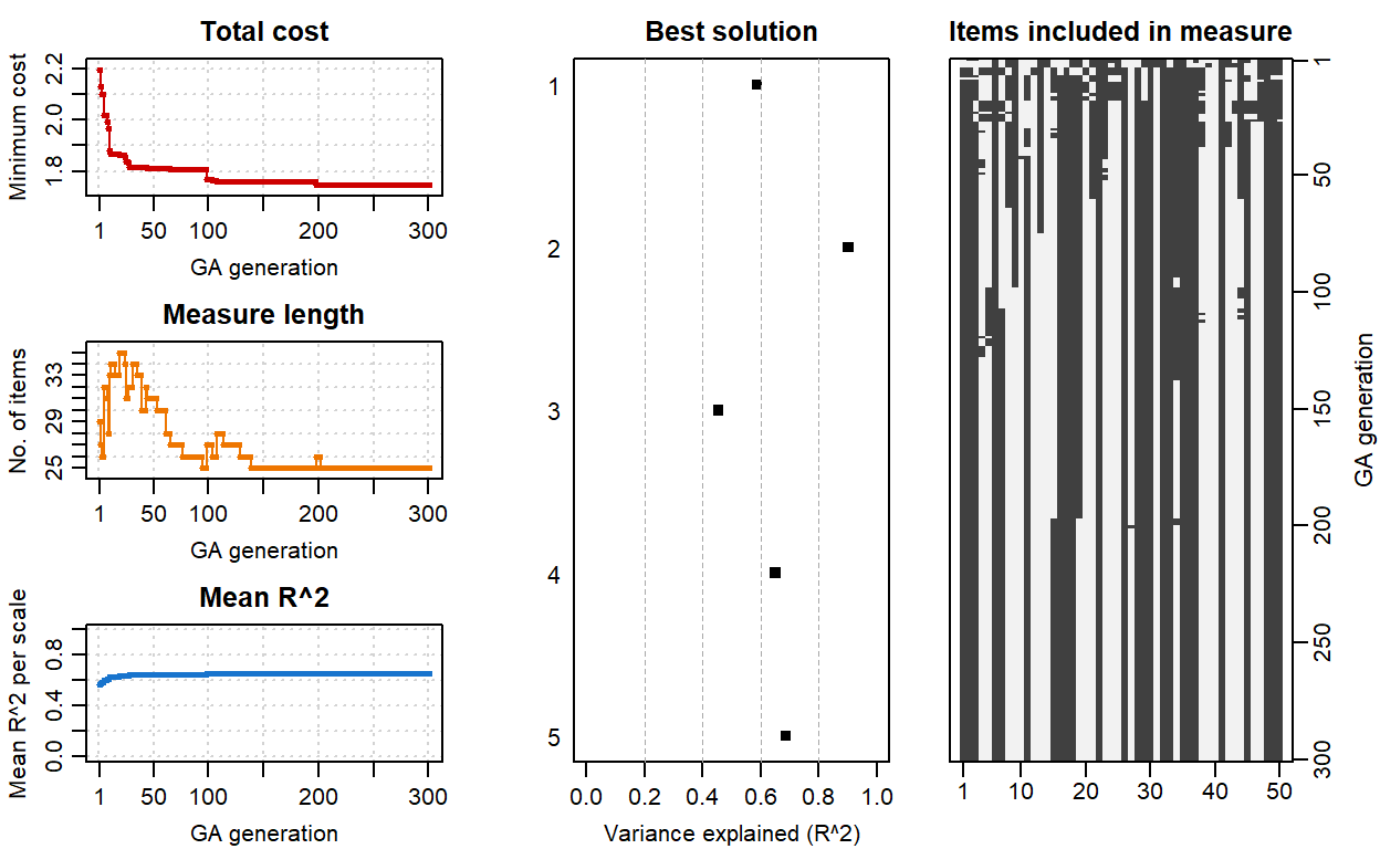
41 45 48 49 50 - We can also request for a summary plot of the Genetic Algorithm below. The plot has total cost, test length, mean of the overall explained variance, explained variance in each dimension, and pattern of items included in each iteration.
Show code
plot(ipip_ga)
Ant Colony Algorithm
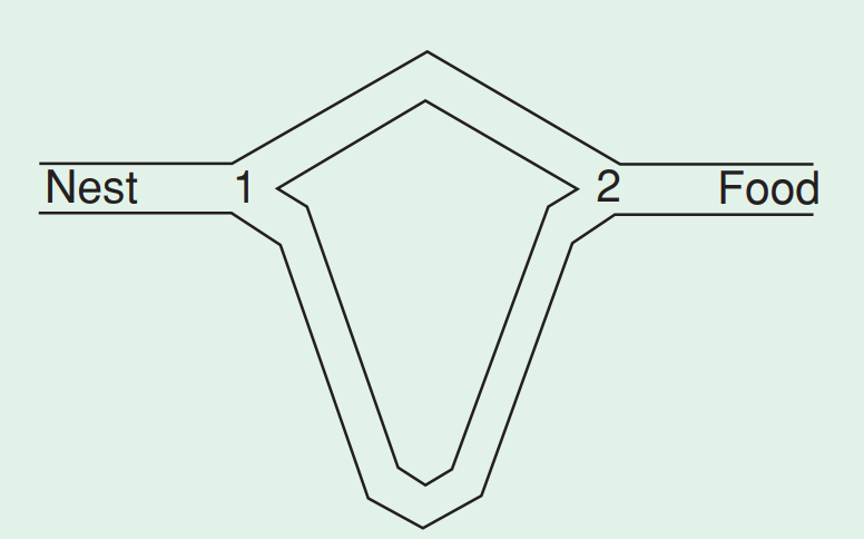
One more way we can shorten our test is using the Ant Colony Optimization (ACO) algorithm. ACO is an optimization method inspired from the foraging behavior of Argentine ants by using virtual ants to find the shortest path to a destination, which is the optimal set of test items for our case (Doringo et al., 2006).
See Figure 2 below for the visual illustration of ACO. There are two routes that lead to the same food source. As ants travel randomly to the food source, they all leave pheromone for others to follow them.
However, given that the upper route is shorter, it receives more pheromone as ants travel back and forth from their nest to the food source more often. The route with more pheromone (i.e., the shorter route) is chosen more by the ants while the longer route gets chosen less as the pheromone evaporates from having less ant.
- We will use the
Shortformpackage to perform test abbreviation with ACO (Raborn & Leite, 2020). We will load the package and subset the data for feasibility. ACO is quite computationally expensive with a large data set. To save time, I subsetted only the first 100 cases of IPIP response data.
  #####                             #######
 #     # #    #  ####  #####  ##### #        ####  #####  #    #
 #       #    # #    # #    #   #   #       #    # #    # ##  ##
  #####  ###### #    # #    #   #   #####   #    # #    # # ## #
       # #    # #    # #####    #   #       #    # #####  #    #
 #     # #    # #    # #   #    #   #       #    # #   #  #    #
  #####  #    #  ####  #    #   #   #        ####  #    # #    #

         Version 0.4.6
             (o<
             //\
             V_/_
Show code
df_survey_aco <- df[1:100, 1:50] #ACO uses dataframe format
- We will also define model structure of the measurement with
lavaansyntax. Here, I defined five dimensions that are measured by 10 items each. In addition to the measurement model, I will also indicate the list of items that measure each dimension.
Show code
model <- " ext =~ EXT1+EXT2+EXT3+EXT4+EXT5+EXT6+EXT7+EXT8+EXT9+EXT10
           est =~ EST1+EST2+EST3+EST4+EST5+EST6+EST7+EST8+EST9+EST10
           agr =~ AGR1+AGR2+AGR3+AGR4+AGR5+AGR6+AGR7+AGR8+AGR9+AGR10
           csn =~ CSN1+CSN2+CSN3+CSN4+CSN5+CSN6+CSN7+CSN8+CSN9+CSN10
           opn =~ OPN1+OPN2+OPN3+OPN4+OPN5+OPN6+OPN7+OPN8+OPN9+OPN10
         "

items <- list(c(paste0("EXT", seq(1, 10))),
              c(paste0("EST", seq(1, 10))),
              c(paste0("AGR", seq(1, 10))),
              c(paste0("CSN", seq(1, 10))),
              c(paste0("OPN", seq(1, 10)))
              )

items
[[1]]
 [1] "EXT1"  "EXT2"  "EXT3"  "EXT4"  "EXT5"  "EXT6"  "EXT7"  "EXT8"
 [9] "EXT9"  "EXT10"

[[2]]
 [1] "EST1"  "EST2"  "EST3"  "EST4"  "EST5"  "EST6"  "EST7"  "EST8"
 [9] "EST9"  "EST10"

[[3]]
 [1] "AGR1"  "AGR2"  "AGR3"  "AGR4"  "AGR5"  "AGR6"  "AGR7"  "AGR8"
 [9] "AGR9"  "AGR10"

[[4]]
 [1] "CSN1"  "CSN2"  "CSN3"  "CSN4"  "CSN5"  "CSN6"  "CSN7"  "CSN8"
 [9] "CSN9"  "CSN10"

[[5]]
 [1] "OPN1"  "OPN2"  "OPN3"  "OPN4"  "OPN5"  "OPN6"  "OPN7"  "OPN8"
[9] "OPN9" "OPN10"- We will create the ACO object with the
antcolony.lavaanfunction. We will set the number of ants to 20, pheromone evaporation rate to 0.5, and fit indices of comparative fit index (CFI), Tucker-Lewis index (TLI), and root mean square error of approximation (RMSEA).
Show code
ipip_ACO <- antcolony.lavaan(data = df_survey_aco, # Response data set
                            ants = 20, # Number of ants
                            evaporation = 0.5, #  % of the pheromone retained after evaporation
                            antModel = model, # Factor model for IPIP
                            list.items = items, # Items for each dimension
                            full = 50, # The total number of unique items in the IPIP scale
                            i.per.f = c(5, 5, 5, 5, 5), # The desired number of items per dimension. The number has to match the number of dimension
                            factors = c('EXT','EST','AGR','CSN','OPN'), # Names of dimensions

                            # lavaan settings - Change estimator to WLSMV
                            lavaan.model.specs = list(model.type = "cfa", auto.var = T, estimator = "WLSMV",
                                                      ordered = NULL, int.ov.free = TRUE, int.lv.free = FALSE,
                                                      auto.fix.first = TRUE, auto.fix.single = TRUE,
                                                      auto.cov.lv.x = TRUE, auto.th = TRUE, auto.delta = TRUE,
                                                      auto.cov.y = TRUE, std.lv = F),

                            steps = 50, # The number of ants in a row for which the model does not change
                            fit.indices = c('cfi', 'tli', 'rmsea'), # Fit statistics to use
                            fit.statistics.test = "(cfi > 0.95)&(tli > 0.95)&(rmsea < 0.06)",
                            max.run = 300) # The maximum number of ants to run before the algorithm stops
 Run number 1.
 Run number 2.
 Run number 3.
 Run number 4.
 Run number 5.
 Run number 6.
 Run number 7.
 Run number 8.
 Run number 9.
 Run number 10.
 Run number 11.
 Run number 12.
 Run number 13.
 Run number 14.
 Run number 15.
 Run number 16.
 Run number 17.
 Run number 18.
 Run number 19.
 Run number 20.
Run number 21. [1] "Compiling results."- After getting the result, we can check our fit indices and the list of items retained by ACO. Item that has “1” indicates that it is selected by the algorithm.
Show code
ipip_ACO[[1]]
          cfi       tli      rmsea mean_gamma EXT1 EXT2 EXT3 EXT4
[1,] 0.968031 0.9638086 0.03537734      0.529    1    0    1    0
     EXT5 EXT6 EXT7 EXT8 EXT9 EXT10 EST1 EST2 EST3 EST4 EST5 EST6
[1,]    1    0    1    0    1     0    0    0    1    0    1    1
     EST7 EST8 EST9 EST10 AGR1 AGR2 AGR3 AGR4 AGR5 AGR6 AGR7 AGR8
[1,]    0    1    0     1    0    1    1    1    1    0    0    1
     AGR9 AGR10 CSN1 CSN2 CSN3 CSN4 CSN5 CSN6 CSN7 CSN8 CSN9 CSN10
[1,]    0     0    1    1    0    0    1    0    0    0    1     1
     OPN1 OPN2 OPN3 OPN4 OPN5 OPN6 OPN7 OPN8 OPN9 OPN10
[1,] 1 0 0 0 1 0 0 1 1 1- We can also request for the summary of lavaan model from the subtest extracted by ACO.
Show code
ipip_ACO$best.model
lavaan 0.6-11 ended normally after 71 iterations

  Estimator                                       DWLS
  Optimization method                           NLMINB
  Number of model parameters                        60

  Number of observations                           100

Model Test User Model:
                                              Standard      Robust
  Test Statistic                               283.962     324.326
  Degrees of freedom                               265         265
  P-value (Chi-square)                           0.202       0.007
  Scaling correction factor                                  1.883
  Shift parameter                                          173.490
simple second-order correction - Next, we can also request for an output of which item is loaded onto which dimension in the new model.
Show code
cat(ipip_ACO$best.syntax)
EXT =~ EXT7 + EXT3 + EXT5 + EXT1 + EXT9
EST =~ EST3 + EST10 + EST6 + EST8 + EST5
AGR =~ AGR8 + AGR4 + AGR3 + AGR2 + AGR7
CSN =~ CSN2 + CSN5 + CSN9 + CSN1 + CSN10
OPN =~ OPN5 + OPN8 + OPN1 + OPN9 + OPN10
- When checking coefficient alpha reliability of the items chosen by ACO, we can see below that the dimension of extraversion, emotional stability, agreeableness, and conscientiousness have satisfactory reliability values.
Show code
 raw_alpha std.alpha   G6(smc) average_r      S/N        ase  mean
 0.8854019  0.886472 0.8729437 0.6096311 7.808396 0.01810261 3.038
       sd  median_r
 1.032285 0.5956059
Show code
 raw_alpha std.alpha  G6(smc) average_r      S/N        ase  mean
  0.819672 0.8179554 0.816637 0.4733049 4.493158 0.02866376 2.962
        sd  median_r
 0.9705544 0.4724666
Show code
 raw_alpha std.alpha G6(smc) average_r      S/N        ase  mean
 0.7890755  0.788927 0.76396 0.4277669 3.737698 0.03327975 3.794
        sd  median_r
 0.7776967 0.4230731
Show code
 raw_alpha std.alpha   G6(smc) average_r      S/N        ase  mean
 0.7009179 0.6928163 0.6664406 0.3108564 2.255382 0.04580886 3.284
        sd  median_r
 0.7914595 0.2909734
Show code
 raw_alpha std.alpha   G6(smc) average_r      S/N        ase  mean
 0.5971511 0.6095035 0.5874082 0.2379028 1.560843 0.06264639 3.802
        sd  median_r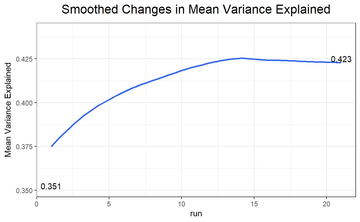
0.6006697 0.2483103- The explained variance plot below shows that ACO was able to increase the amount of variance explained by the model.
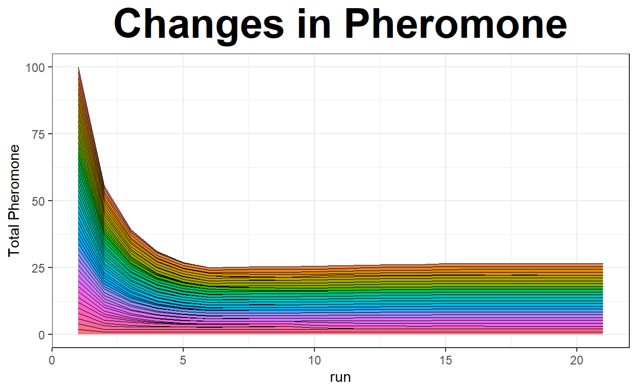
- We can also request for the pheromone plot with the argument
type=""pheromone. This will allow us to see the amount of pheromone used by our virtual ants.
Conclusion
This post demonstrated several ways we can reduce the number of test items whether through the traditional method of reliability examination, Genetic Algorithm, or ACO. Many psychological assessment provides helpful insights to clinicians, educators, and the examinee themselves with helpful information. However, some tests are quite lengthy that they fatigue the examinee out before; for example, the Minnesota Multiphasic Personality Inventory-2 Restructured Form (MMPI-2-RF) has 338 items. Genetic Algorithm and ACO may be useful to reduce the number of test items to the optimal level while retaining accuracy and representativeness of the test.
However, note that the two algorithms are not silver bullets. We cannot just apply them to every test without consulting the literature, test developers, test users, and other relevant stakeholders first. After reducing the number of test items, researchers should check if the remaining items are representative to the measured construct and perform a pilot testing to examine if the test serves its intended purpose. As always, thank you very much for reading this!