Introduction
In my previous post on ensemble machine learning models, I mentioned that one major drawback in the artificial intelligence (AI) field is the black box problem, which hampers interpretability of the results from complex algorithms such as Random Forest or Extreme Gradient Boosting. Not knowing how the algorithm works behind the prediction could reduce applicability of the method itself as the audience can’t fully comprehend the result and therefore unable to use it to inform their decisions; this problem could therefore damage trust from the stakeholders (users, policy makers, general audience) to the field as well (McGovern et al., 2019).
On the developer’s side, fully understanding the machine learning models through the explanable approach (aka the white-box approach) allows developers to identify potential problems such as data leakage in the algorithm and fix (or debug) it with relative ease (Loyola-Gonzalez, 2019). Further, knowing which variable affects the prediction the most can inform feature engineering to reduce model complexity and direct future data collection as well by focusing on collecting the variables that matter (Becker & Cook, 2021).
On stakeholder’s side, it is important to emphasize model explanability especially in industries such as healthcare, finances, and military to foster trust between the people inside and outside of the field that could lead to the extent that the result is used to inform decisions made by humans such as financial credit approval (Becker & Cook, 2021; Loyola-Gonzalez, 2019). Clearly Understanding how, where, and why the model also benefits the model itself as users are able to identify potential problems in its performance and provide the develoeprs with their feedback (Velez et al., 2021).
The above examples knowing how to extract human-understandable insights from a complex machine learning model is important, especially in social science data where the theoretical part is as important as the methodological and the practical part. For that reason, I will be applying the methods of Explanable Artificial Intelligence (XAI) to extract interpretable insights from a classification model that predicts students’ grade repetition. We will begin by setting up the environment as usual.
Show code
import pandas as pd
import matplotlib.pyplot as plt
import seaborn as sns
from collections import Counter

from imblearn.combine import SMOTEENN

from sklearn.manifold import TSNE
from sklearn.model_selection import train_test_split
from sklearn.model_selection import RepeatedStratifiedKFold
from sklearn.model_selection import cross_val_score
from sklearn.ensemble import RandomForestClassifier

from sklearn.metrics import accuracy_score

import warnings
warnings.filterwarnings("ignore")

RANDOM_STATE = 123- I will be using the same data set as my previous post about statistical learning, namely the Programme for International Student Assessment (PISA) 2018 (OECD, 2019). However, the set of variables that I am examining will be different as PISA contains several school-related variables that can be shifted as the researcher sees fit. For this post, I will predict students’ class repetition from 25 predictors (or features as called in the field of machine learning) such as students’ socio-economic status, history of bullying involvement, and their learning motivation. The data is collected from Thai student in 2018.
Show code
df = pd.read_csv("PISA_TH.csv")

X = df.drop('REPEAT', axis=1)
y = df['REPEAT']

df.head()
REPEAT ESCS DAYSKIP ... Invest_effort WEALTH Home_resource
0 0 -0.7914 1 ... 6 0.0721 -1.4469
1 0 0.8188 1 ... 8 -0.3429 1.1793
2 0 0.4509 1 ... 10 0.3031 1.1793
3 0 0.7086 1 ... 10 -0.5893 -0.1357
4 0 0.8361 1 ... 10 0.5406 1.1793
[5 rows x 25 columns]Addressing Sample Imbalance
The problem is that our targeted variable is imbalance; that is, the number of students who repeated a class is smaller than the number of students who did not. This situation makes sense in the real-world data as normal samples are usually more prevalent than the abnormal ones, but it is undesirable in the machine learning scenario as the model could recognize minority samples as unimportant and therefore disregard them as noises (Chawla et al., 2022). As a result, the model could give misleadingly optimistic performance on classification datasets as it classifies only students who did not repeat a class.
See the t-Distributed Stochastic Neighbor Embedding (tSNE) plot below for the visualization. There isn’t much samples of repeaters in contrary to non-repeater students. Plus, the pattern is not prominent enough as the blut dots (repeaters) stay very close to the red dots (non-repeaters). This could make the pattern difficult to be learned by the machine due to its ambiguity. One way we can mitigate this problem is to perform data augmentation via oversampling and undersampling, which synthesizes more minority samples and deletes or merges majority samples to improve performance of the machine (Budhiman et al., 2019; Wong et al;., 2016).
Show code
Counter(y)Counter({0: 8044, 1: 589})Show code
tsne = TSNE(n_components=2, random_state=RANDOM_STATE)

TSNE_result = tsne.fit_transform(X)

plt.figure(figsize=(12,8))
sns.scatterplot(TSNE_result[:,0], TSNE_result[:,1], hue=y, legend='full', palette="hls")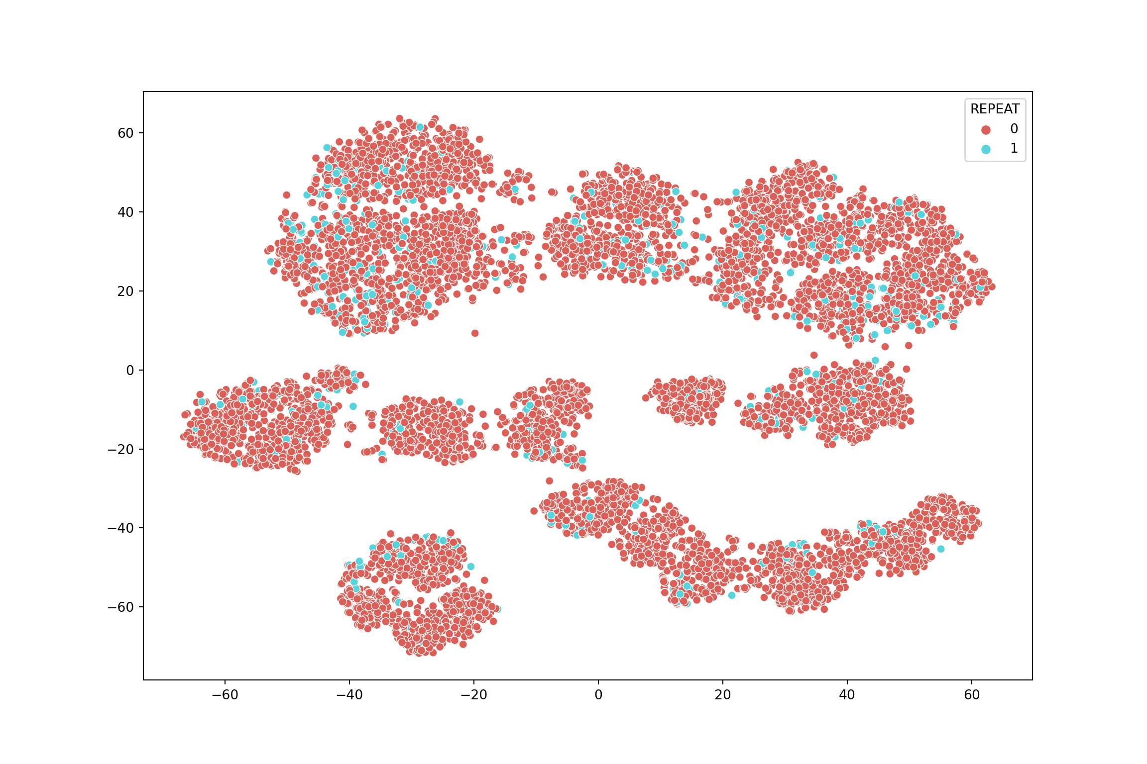
To balance the data, I will use both oversampling and undersampling. Normal oversampling methods duplicates minority samples for more sample size; however, this approach does not add any more information to the model (more of the same, basically). Instead, we can synthesize minority samples by creating samples that are similar to the existing minority samples; this technique is named as Synthetic Minority Oversampling TEchnique (SMOTE) (He and Ma, 2013).
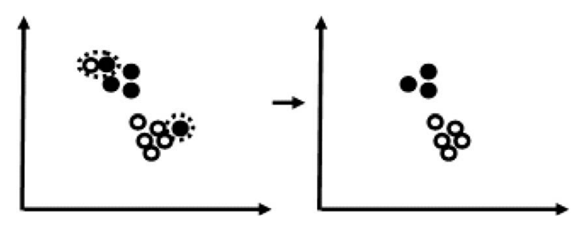
Also, we can further enhance the effectiveness of SMOTE by adding undersampling into the process (Chawla et al., 2022). Instead of randomly delete our majority samples, we will use the Edited Nearest Neighbor (ENN) method, which deletes data points based on their neighbors to make the difference between majority and minority samples (Ludera, 2021). The combination of these two techniques is called SMOTEENN See Figure 1 for the example of ENN from Guan et al., (2009).
Show code
smote_enn = SMOTEENN(random_state=RANDOM_STATE, sampling_strategy = 'minority', n_jobs=-1)

X_resampled, y_resampled = smote_enn.fit_resample(X, y)

Counter(y_resampled)
Counter({1: 8040, 0: 4794})Show code
tsne = TSNE(n_components=2, random_state=RANDOM_STATE)

TSNE_result = tsne.fit_transform(X_resampled)

plt.figure(figsize=(12,8))
sns.scatterplot(TSNE_result[:,0], TSNE_result[:,1], hue=y_resampled, legend='full', palette="hls")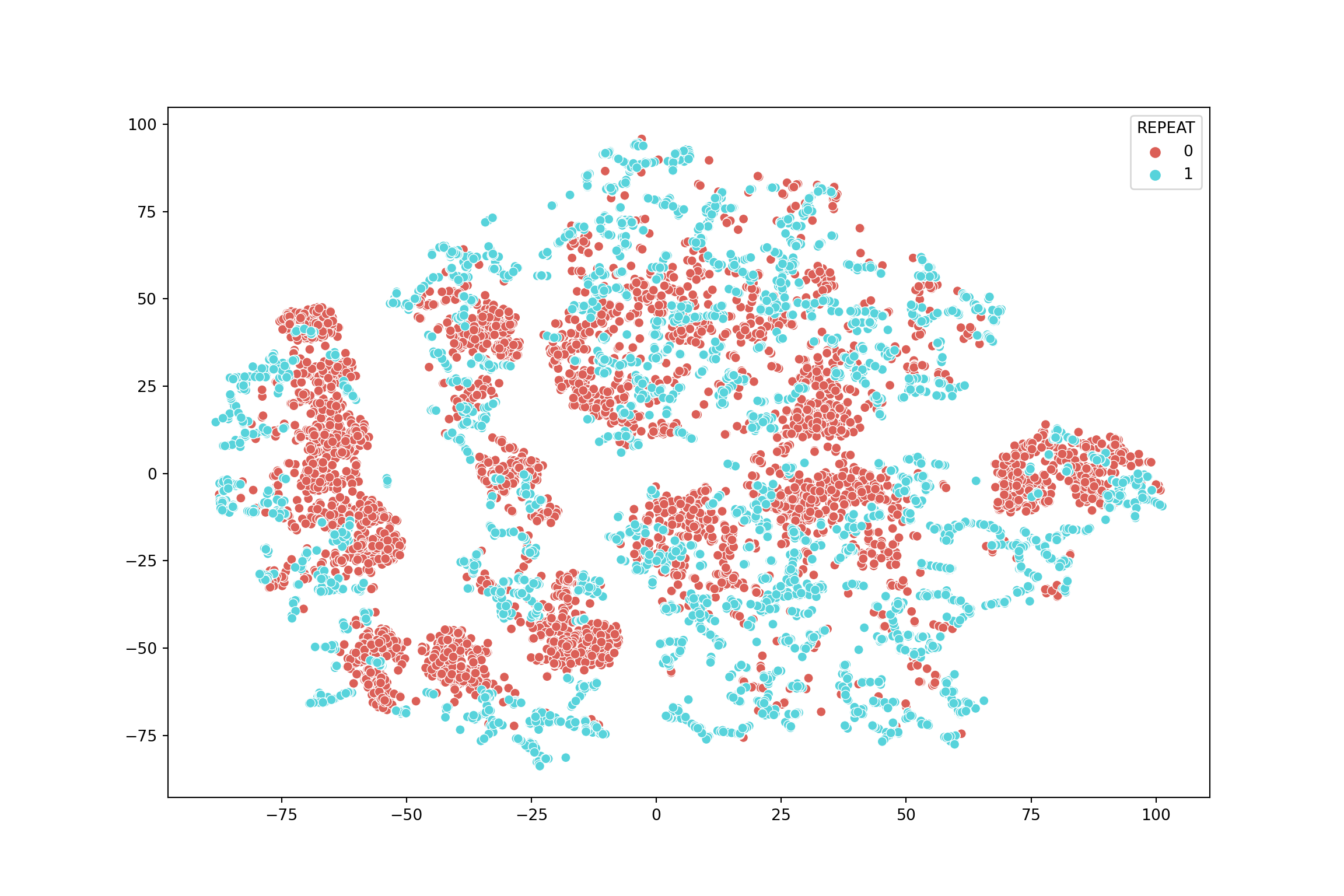
- The second tSNE plot shows a more noticable pattern between student repeaters and non-repeaters. The number of repeaters is increased while the number of non-repeaters is decreased. Next, we can put our augmented data into the Random Forest model for prediction.
Random Forest Ensemble
- We will be splitting the data set into a training and a testing set as usual. For a quick recap, Random Forest is a machine learning model that consists of several unique and uncorrelated decision trees; hence the word Random in its name. Those trees work together to improve the predictive accuracy of that dataset than a single decision tree (Kubat, 2017). The model will be evaluated with the repeated stratified 10-folds technique to test our model prediction on different sets of unseen data to ensure its accuracy, especially in the case of imbalanced data set.
Show code
CV = RepeatedStratifiedKFold(n_splits=10, n_repeats=2, random_state=RANDOM_STATE)


X_train, X_test, y_train, y_test = train_test_split(X_resampled, y_resampled, test_size = 0.30,
                                                    random_state = RANDOM_STATE)
Show code
# random forest model creation
clf_rfc = RandomForestClassifier(random_state=RANDOM_STATE)
clf_rfc.fit(X_train, y_train)

# predictionsRandomForestClassifier(random_state=123)Show code
rfc_predict = clf_rfc.predict(X_test)

rfc_cv_score = cross_val_score(clf_rfc, X_resampled, y_resampled, cv=CV, scoring='roc_auc')

print("=== All AUC Scores ===")
=== All AUC Scores ===Show code
print(rfc_cv_score)[0.98907675 0.99357898 0.99228597 0.99276793 0.99409399 0.99378369
0.9931644 0.9901627 0.98967714 0.99287747 0.99384328 0.99252177
0.99452348 0.99187137 0.99040419 0.99201929 0.9896265 0.99140778
0.99115331 0.99457436]Show code
print('\n')Show code
print("=== Mean AUC Score ===")=== Mean AUC Score ===Show code
print("Mean AUC Score - RandForest: ", rfc_cv_score.mean())Mean AUC Score - RandForest: 0.9921707177188173Show code
#define metrics for normal RF
from sklearn import metrics

y_pred_proba_rf = clf_rfc.predict_proba(X_test)[::,1]
fpr_rf, tpr_rf, _ = metrics.roc_curve(y_test,  y_pred_proba_rf)

auc_rf = metrics.roc_auc_score(y_test, y_pred_proba_rf)
plt.plot(fpr_rf,tpr_rf, label="AUC for Random Forest Classifier = "+str(auc_rf.round(3)))
[<matplotlib.lines.Line2D object at 0x000001EA9D9FA340>]Show code
plt.legend(loc="lower right")<matplotlib.legend.Legend object at 0x000001EA9D9FA220>Show code
plt.ylabel('True Positive Rate')Text(0, 0.5, 'True Positive Rate')Show code
plt.xlabel('False Positive Rate')
Text(0.5, 0, 'False Positive Rate')Show code
plt.title("Receiver-Operator Curve (ROC)")Text(0.5, 1.0, 'Receiver-Operator Curve (ROC)')Show code
plt.show()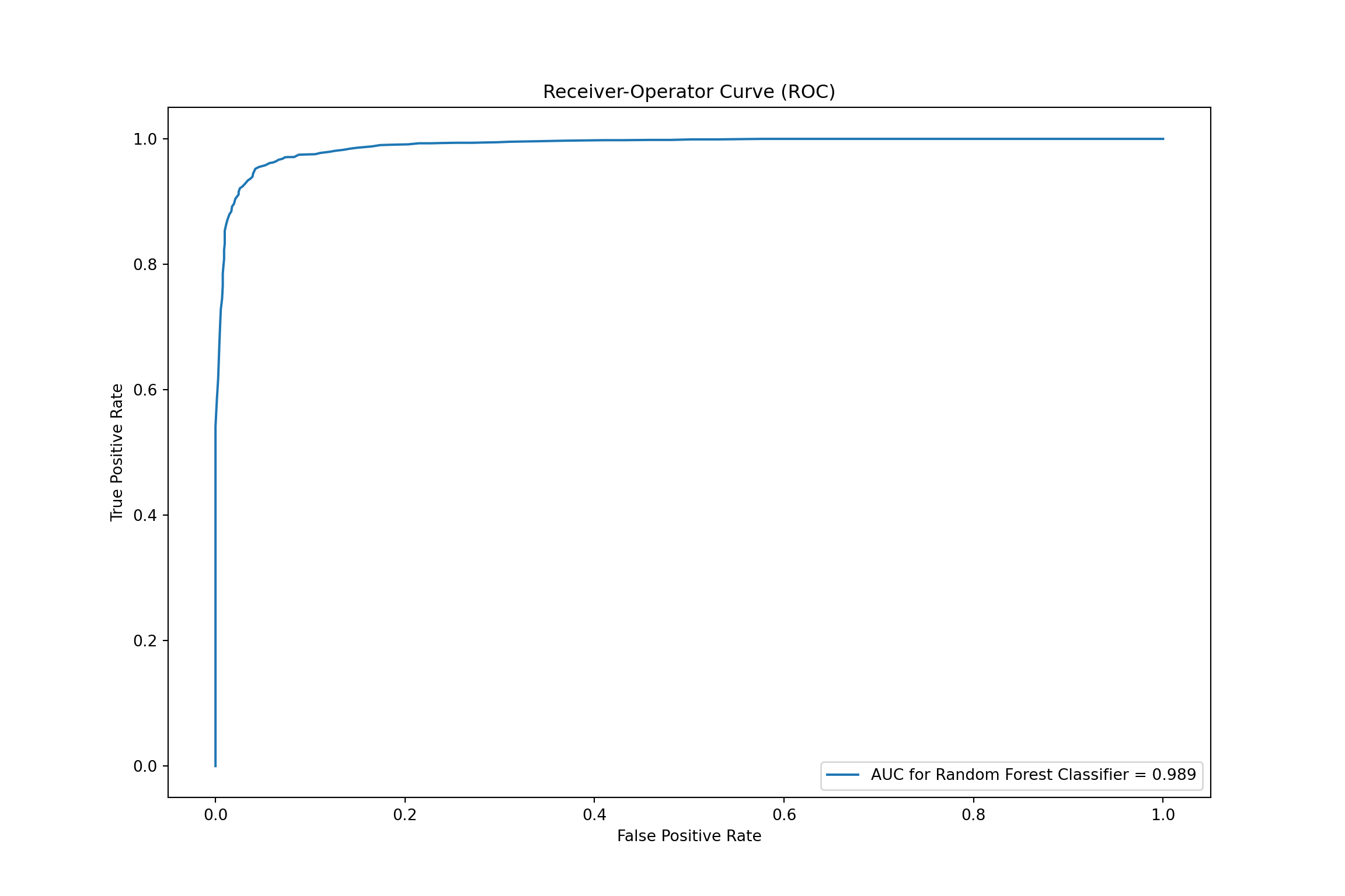
- The results will be evaluated with the Receiver Operator Characteristic (ROC) curve, which shows the diagnostic ability of binary classifiers. One approach to use ROC is to evaluate its Area Under Curve (AUC), which measures of the ability of a classifier to distinguish between classes and is used as a summary of the ROC curve. The higher the AUC, the better the performance of the model at distinguishing between the positive and negative classes. The mean of 20 rounds of testing (randomly splitting the data into 10 stratified parts, repeated it for 2 times) looks good is around 0.99, meaning that there is a 99% chance that the model is able to correctly predict which student is a reapeater and which is not based on the data used to train the machine. Now we know that the model works well with our data, let us move on to interpreting it with XAI techniques.
Explaining AI
- XAI is a set of methods that allows a machine learning model and its results understandable to human in terms of how it works in terms of prediction, including the impace of variables to the prediction results (Gianfagna & Di Cecco, 2021). The XAI methods that we will extract insights are permutation importance, partial dependence plot, and Shapley Additive explanations (SHAP) values.
Permutation Importance
- One of the most basic questions we might ask of a model is: What features have the biggest impact on predictions? This quention could be answered through the examination of feature importance. There are multiple ways to measure feature importance. One way is to extract the feature importance plot from the model itself as demonstrated below.
Show code
# Create a pd.Series of features importances
importances_rf = pd.Series(clf_rfc.feature_importances_, index = X_resampled.columns)

# Sort importances_rf
sorted_importance_rf = importances_rf.sort_values()

#Horizontal bar plot
sorted_importance_rf.plot(kind='barh', color='lightgreen');
plt.xlabel('Feature Importance Score')
Text(0.5, 0, 'Feature Importance Score')Show code
plt.ylabel('Features')Text(0, 0.5, 'Features')Show code
plt.title("Visualizing Important Features")Text(0.5, 1.0, 'Visualizing Important Features')Show code
plt.show()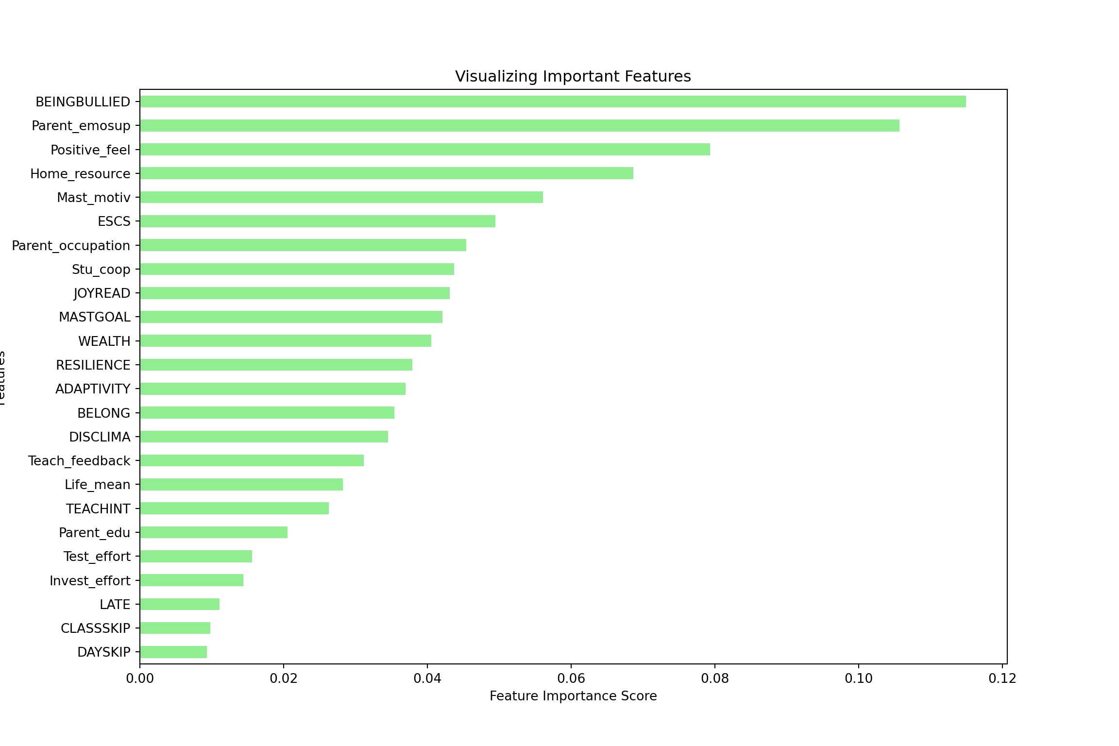
- Another way, which we will focus on in this post, is to use the permutation importance score from the area of XAI. Permutation importance is calculated by asking the following question: “If I randomly shuffle a single column of the validation data, leaving the target and all other columns in place, how would that affect the accuracy of predictions in that now-shuffled data?”. Randomly re-ordering a single column should cause less accurate predictions, since the resulting data no longer corresponds to anything observed in the real world. Model accuracy especially suffers if we shuffle a column that the model relied on heavily for predictions. In our case, if we mess with the “BEINGBULLIED” variable, the model would be severely affected by the reduced prediction accuracy. The same would happen to the variable “Parent_emosup”, “Positive_feel” and so forth as well.
Show code
import eli5
from eli5.sklearn import PermutationImportance

FEATURES = X_test.columns.tolist()

perm = PermutationImportance(clf_rfc, random_state=RANDOM_STATE).fit(X_test, y_test)
eli5.show_weights(perm, feature_names = FEATURES, top = 10)
<IPython.core.display.HTML object>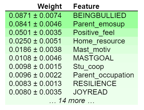
The permutation importance results are consistent with the feature importance score we extracted from the model. The values towards the top are the most important features, and those towards the bottom matter least. The first number in each row shows how much model performance decreased with a random shuffling (in this case, using “accuracy” as the performance metric). Like most things in data science, there is some randomness to the exact performance change from a shuffling a column. We measure the amount of randomness in our permutation importance calculation by repeating the process with multiple shuffles. The number after the ± measures how performance varied from one-reshuffling to the next.
In our example, the most important feature was “BEINGBULLIED”, which is the index of exposure to bullying. The index was constructed from questions that ask if students have experienced bullying in the past 12 months from statements such as “Other students left me out of things on purpose”; “Other students made fun of me”; “I was threatened by other students”. Positive values on this scale indicate that the student was more exposed to bullying at school than the average student in OECD countries; negative values on this scale indicate that the student was less exposed to bullying at school than the average student across OECD countries. This result is consistent with the literature that students’ grade repetition is associated with the likelihood of being bullied (Lian et al., 2021; Ozada Nazim & Duyan, 2019)
Partial Dependence Plots
While feature importance shows what variables most affect predictions, partial dependence plots show how a feature affects predictions. For our case, partial dependence plots can be used to answer questions such as “Controlling for all variables, what impact does the index of exposure to bullying have on the prediction of grade repetition?”. The interpretation of partial dependence plot is somewhat similar to the interpretation of linear or logistic regression. On this plot, The y axis is interpreted as change in the prediction from what it would be predicted at the baseline or leftmost value. A blue shaded area indicates level of confidence.
The plot below indicates that being subjected to bullying (as reflected by having positive value of the variable) increases the likelihood of students to repeat a grade. Positive values in this index indicate that the student is more exposed to bullying at school than the average student in OECD countries. Negative values in this index indicate that the student is less exposed to bullying at school than the average student in OECD countries; therefore, having zero does not mean students did not experience any form of bullying, but rather experiencing bullying to some degree (i.e., being bullied a bit). However, the predicting power does not change much after 0, meaning that the amount of exposure to bullying does not matter in predicting students’ grade repetition.
Show code
from pdpbox import pdp

pdp_bullied = pdp.pdp_isolate(model=clf_rfc, dataset=X_test, model_features=FEATURES, feature='BEINGBULLIED')

pdp.pdp_plot(pdp_bullied, 'BEINGBULLIED')
(<Figure size 1500x950 with 2 Axes>, {'title_ax': <AxesSubplot:>, 'pdp_ax': <AxesSubplot:xlabel='BEINGBULLIED'>})Show code
plt.show()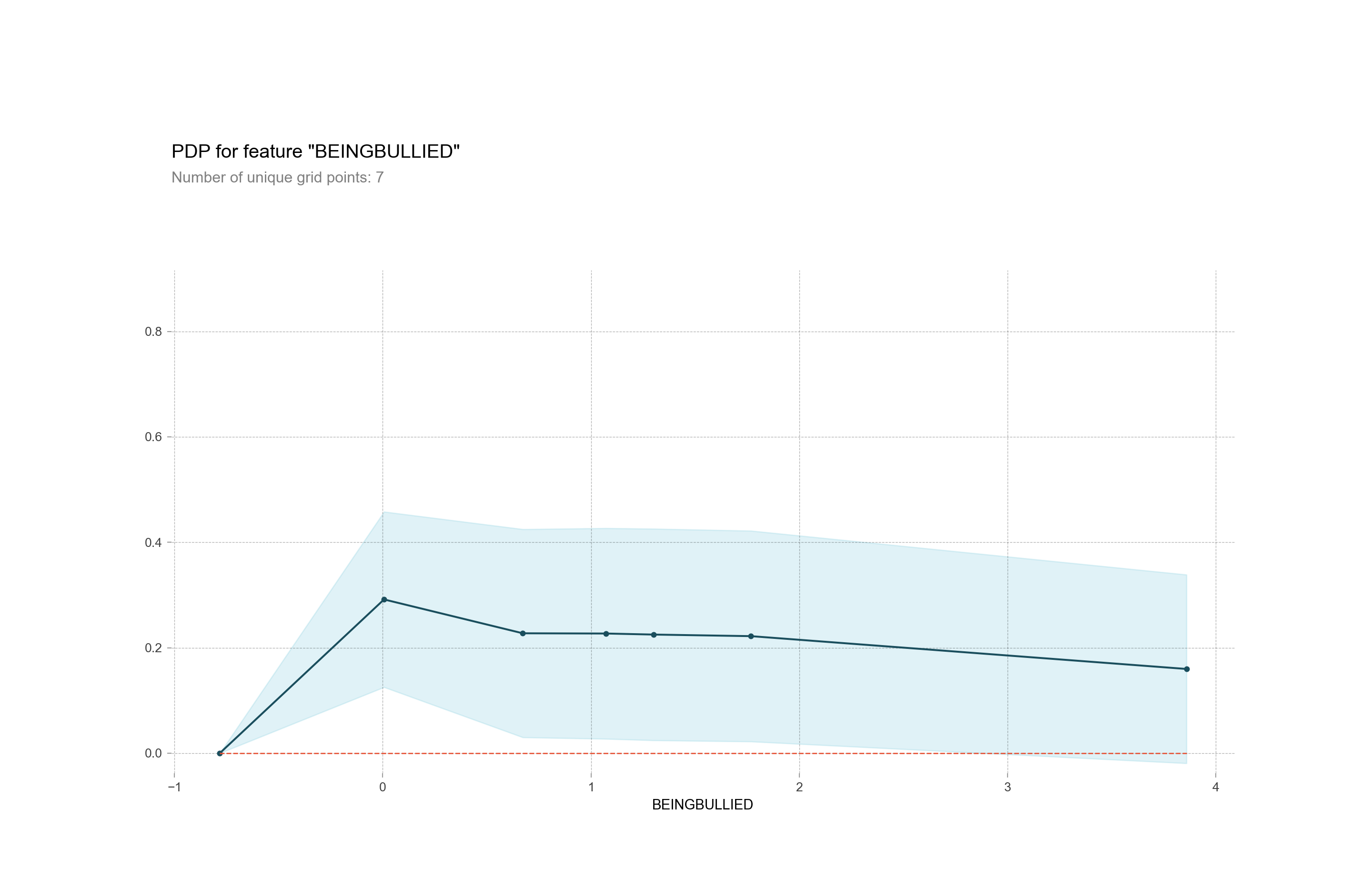
- Partial Dependence Plots can also be used to examine interactions between variables as well. The graph below shows predictions for any combination of students’ exposure to bullying and the amount of emotional support from parents. The prediction power is highest when students score 0 in the index of exposure to bullying (i.e., being bullied a bit) and having scores on the index of parents’ emotional support between -1.7 to +0.5. Positive values on this scale mean that students perceived greater levels of emotional support from their parents than did the average student across OECD countries while negative value means otherwise. Having higher exposure to bullying reduces prediction power of the model as indicated by the changing color from yellow to green, and when the score in the index of emotional support reaches 1, the score of the exposure to bullying index becomes less matter as the prediction power reduces.
Show code
features_to_plot = ['BEINGBULLIED', 'Parent_emosup']

inter1  =  pdp.pdp_interact(model=clf_rfc, dataset=X_test, model_features=FEATURES, features=features_to_plot)

pdp.pdp_interact_plot(pdp_interact_out=inter1, feature_names=features_to_plot, plot_type='contour')
(<Figure size 750x950 with 3 Axes>, {'title_ax': <AxesSubplot:>, 'pdp_inter_ax': <AxesSubplot:xlabel='BEINGBULLIED', ylabel='Parent_emosup'>})Show code
plt.show()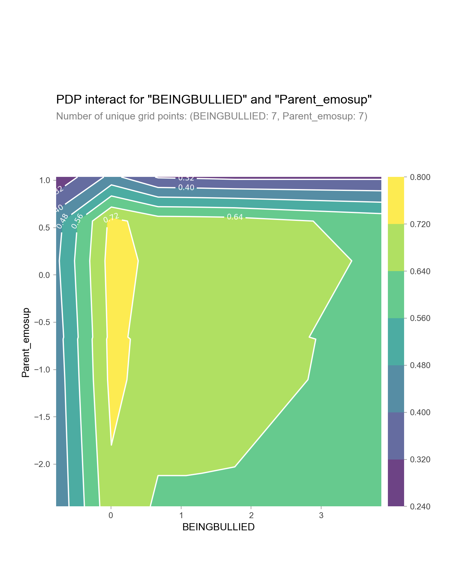
SHAP Values
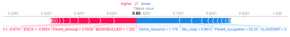
Finally, SHAP value allows us to interpret the prediction at a fine-grained level to the components of individual predictions to show the impact of each feature. For our case, CHAP value can be used to answer questions like “On what basis did the model predict that student A is likely to repeat a grade?”. The plot is quite straightforward to interpret. The red part shows what increases the likelihood of repeating a grade, and the blue part shows what decreases the likelihood of repeating a grade.
On the plot below, the prediction is at the base alue of 0.60, meaning that it is the average of the model output. For this particular student, their likelihood to repeat a grade is increased by being exposed to bullying (BEINGBULLIED), having mediocre emotional support from parents (Parent_emosup), and having poor overall social standing as indicated by -0.9 the variable the index of socio-economic, social and cultural status (ESCS). However, the likelihood is decreased by their educational resources at home (Home_resource), having cooperative class (Stu_coop), their parents’ occupational status (Parent_occupation), and having low record of class skipping (CLASSKIP).
SHAP Summary Plot
In addition to the breakdown of each individual prediction, we can also visualize groups of SHAP values with SHAP summary plot and SHAP dependence contribution plot. SHAP summary plots give us an overview of feature importance and what is driving the prediction. This plot is made of many dots. Each dot has three characteristics as follows: a) horizontal location (the x-axis) that indicates whether the effect of that value caused a higher or lower prediction; b) vertical location (the y-axis) that indicates the variable name, in order of importance from top to bottom. c) Gradient color indicates the original value for that variable. In booleans (i.e., yes/no variable), it will take two colors, but in number it can contain the whole spectrum.
For example, the left most point in the ‘Parent_emosup’ row is red in color, meaning that for that particular student, having greater levels of emotional support from their parents reduces their likelihood of repeating a grade by roughly 0.3. Seeing variables have a wide spread in range can be inferred that permutation importance is high; however, it is best to use permutation importance to measure which variable is important to the prediction.
Some features such as
Home_resource(educational resource at home) have reasonably clear separation between the blue and pink dots, which implies a straightforward meaning that the increase in the variable value lower (i.e., more resource) the likelihood of repeating a grade while the decrease in educational resource impacts the variable in the other direction (higher chance to repeat a grade).However, some variables such as
Stu_coop(the degree of cooperativeness within classrooms) have blue and pink dots jumbled together, suggesting that the increase in this variable leads to higher predictions, and other times it leads to a lower prediction. In other words, both high and low values of the variable can have both positive and negative effects on the prediction. The most likely explanation for this “jumbling” of effects is that the variable (in this caseStu_coop) has an interaction effect with other variables. For example, there may be some situations where cooperating with other students lead to social loafing - when stduents contribute less effort when working as a group, and therefore learns less. This interaction needs further investigation.
Show code
shap_values_summary = explainer.shap_values(X_test)
shap.summary_plot(shap_values[1], X_test)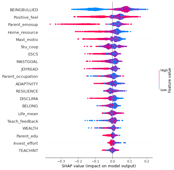
SHAP Dependence Contribution Plot
The earlier Partial Dependence Plots to show how a single feature impacts predictions. This is insightful and relevant for many real-world use cases. The interpretation is also friendly to non-technical audience as well. However, there is a lot that we still don’t know; for example, what is the distribution of effects? Is the effect of having a certain value pretty constant, or does it vary a lot depending on the values of other feaures. SHAP dependence contribution plots provide a similar insight to the partial dependence plot, but they add a lot more detail. The plot shows scatter dots that explain how the effect a single feature has on the predictions made by the model. The plot can be read as follows: a) The x-axis is the value of the feature; b) The y-axis is the SHAP value for that feature, which represents how much knowing that feature’s value changes the output of the model prediction; c) The color corresponds to a second feature that may have an interaction effect with the feature we are plotting.
The plot below shows the relatively flat trend of the
BEINGBULLIEDfeature, meaning that this variable does impact the prediction regardless of the value; this trend is consistent with the partial dependence plot shown earlier in the post. However, there is a sign of interaction as there are points with similar value that produce different outcome. See the left of the 2D pane, for example. For some students, being less exposed to bullying gives them more chance to repeat a grade while some students got less chance. There might be other features that interact with this variable.While the primary trend is that being bullied increases the chance of repeating a grade , there are some variations that can be explained by the interaction of features as well. For a concrete explanation, see the right of the 2D pane. Being positioned overthere means that those students experience a lot of bullying, but their chance of repeating a grade is relatively lower than those who experience less bullying. One explanation is that some of those students have positive feelings for themselves (indicated by the red color), which could make them more resilient toward being bullied.
Show code
shap.dependence_plot('BEINGBULLIED', shap_values_summary[1], X_test, interaction_index="Positive_feel")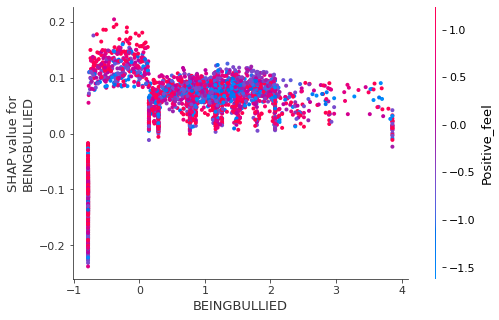
Conclusion
- What we have done so far is making a prediction with a Random Forest
Ensemble model, which has high predictive power at the price of being
challenging to explain due to its complexity (Zhang &
Wang, 2009). XAI tools such as permutation importance, partial
dependence plot, and SHAP values, allow us to understand outputs of the
model at various levels from the overall picture to fine-grained
individual cases. Knowing how predictions are made also allow
establishes venues for future studies as well. XAI results are important
to bridge the knowledge gap between technical (e.g., developers) and
non-technical (e.g., customers, users) audiences, which could build
trust and confidence when putting the AI models into the actual use. XAI
also helps an organization develop a responsible approach to AI
development by avoiding the reliance on results that we do not
understand to inform our decisions.
- However, note that XAI is not perfect. Its results are context-dependent, meaning that if the context changes, so does the result (de Brujin et al., 2021). The prediction and how it happens can only be used as a factor to be considered along with other lines of evidence such as expert opinion, counter explanations, and potential consequences. Regardless, XAI is still a useful too to have in expanding the knowledge we get from machine learning. Thank you very much for reading!